Business and Economic Statistics

Introduction

Descriptive Statistics - Method that focus on the collection, preesentation and characterization of a set of data in order to property describe the various features of data sets

Population - the totality of items or things under consideration

Parameter - summary measure that describes a characteristic of an entire population

Sample - portion of population that is selected for analysis

Statistic - summary measure computed from sample data that is used to describe or estimate a characteristic of the entire population

Reasons for obtaining Data

1. Provide necessary input to a survey, study

2. Measure performance of an ongoing service or production process

3. Evaluate conformance to standards

4. Assist in formulating alternative courses of action in a decision-making process

5. Satisfy our curiosity

Sources of Data

1. Government, industrial or individual sources

2. Experiment

3. Survey

4. Observational Study

Types of Data

1. Categorical random variables, e.g. Yes / No Question

2. Numerical random variables, e.g. how much money will you spend every week?

3. Discrete random variables - arise from counting process

4. Continuous random variables - arise from a measuring process

Organizing Data

Ordered Array - sequence of raw data in rank order from smallest to largest

Stem and Leaf Display

Tables and Charts (Numerical)

Width of class interval = Range / no. of desired class groupings

Main advantage of using summary table is that the major data characteristics can become immediately clear to the reader.

Histogram - constructed in the boundaries of each class

Cumulative Frequency Polygon (Ogive)

Tables and Charts (Categorical)

Summary Table, Bar chart, Pie Chart, Pareto Diagram

Graphical Excellence

1. well-designed presentation of data that provides substance, statistics and design

2. Communicate complex ideas with clarity, precision and efficiency

3. Give the viewer the largest number of ideas in the shortest time with the least ink

4. Always involve several dimensions

5. Telling the truth about the data

Chart junk is a decoration that is redundant data-ink

Focus - Labelling, zero value in X axis and Y axis, Title, Time series

Numerical Descriptive measures

Measures of Central Tendency

• Mean

• Median - (n+1)/2  ranked observation

• Mode

• Quartiles - q (n+1) / 4 ranked observation

• Geometric Mean -  {(1+R) X (1+R) ...... X (1+Rn) } to the power 1 -n, - 1

Measures of Variation

• Range = Largest value - Smallest value

• Interquartile Range = Q3 - Q1

• Sample variance = (value - Mean ) square / n -1

• Sample S.D. = Square root (Sample variance)

• Population Mean = Sample Mean

• Population variance = (value - Mean ) square / N

• Population S.D. = Square root (Population variance)

          The variance and the S.D. measure the "average scatter" around the mean

More spread out, Larger range, Interquartile range, variance, the standard deviation

More concentrated, or homogeneous, the smaller the dispersion

If the observation are all the same, the dispersion will be zero.

Coefficient of variation - Sample S.D. / Sample Mean X 100 %

The higher the risk category the larger the relative size of the average spread around the mean is to the mean.

Shape

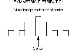
Symmetrical

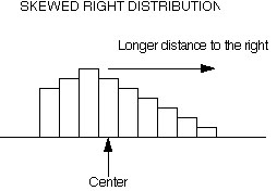
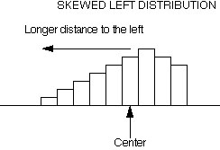
Asymmetrical / Skewed

Mean > Median: positive or right-skewness (the peak distort to the left) - mean is increased by some unusually high values

Mean = Median: Symmetry, or zero-skewness (the peak in the central)

Mean < Median: negative or left-skewness (the peak distort to the right) - mean is reduced by some unusually low values

The skewness for a normal distribution is zero, and any symmetric data should have a skewness near zero.

Negative values for the skewness indicate data that are skewed left and positive values for the skewness indicate data that are skewed right. By skewed left, we mean that the left tail is heavier than the right tail. Similarly, skewed right means that the right tail is heavier than the left tail.

Skewness measures the coefficient of asymmetry of a distribution. A risk-averse investor does not like negative skewness

Box-and-Whisker Plot

- graphical representation of the data based on the five-number summary

Importance of indicating the shape, center, and spread when describing a distribution

You can think of this in terms of summaries of various lengths describing the data, starting with the shortest summary, which would
be some sort of "typical" value or measure of center.  Then you might wonder if all the data are typical or if there is a lot of scatter, so step 2 might be a measure of variability. 

Finally, shape helps you to put these into perspective and choose appropriate summaries.  An approximate normal distribution has most of the data clumped around the center, and the mean and s.d. are good summaries.  A distribution that is highly skewed and/or has a lot of outliers might better be described with a median and IQR.  A bimodal distribution usually is not well characterized by ONE typical value.  Etc.