Communication Protocols
Approximately 30 years ago, communication
protocols were developed so that individual stations could be connected
to form a local area network (LAN). This group of computers and other
devices, dispersed over a relatively limited area and connected by a
communications link, enabled any station to interact with any other on
the network. These networks allowed stations to share resources, such as
laser printers and large hard disks. This chapter and Chapter 2 discuss
the communication protocols that became a set of rules or standards
designed to enable these stations to connect with one another and to
exchange information. The protocol generally accepted for standardizing
overall computer communications is a seven-layer set of hardware and
software guidelines known as the Open Systems Interconnection (OSI)
model. Before one can accurately define, implement, and test (hack into)
security policies, it is imperative to have a solid understanding of
these protocols. These chapters will cover the foundation of rules as
they pertain to TCP/IP, ARP, UDP, ICMP, IPX, SPX, NetBIOS, and NetBEUI.
 A
Brief History of the Internet
A
Brief History of the Internet
During the 1960s, the U.S. Department of
Defense’s Advanced Research Projects Agency (ARPA, later called DARPA)
began an experimental wide area network (WAN) that spanned the United
States. Called ARPANET, its original goal was to enable government
affiliations, educational institutions, and research laboratories to
share computing resources and to collaborate via file sharing and
electronic mail. It didn’t take long, however, for DARPA to realize the
advantages of ARPANET and the possibilities of providing these network
links across the world. By the 1970s, DARPA continued aggressively
funding and conducting research on ARPANET, to motivate the development
of the framework for a community of networking technologies. The result
of this framework was the Transmission Control Protocol/Internet
Protocol (TCP/IP) suite. (A protocol is basically defined as a set of
rules for communication over a computer network.) To increase acceptance
of the use of protocols, DARPA disclosed a less expensive implementation
of this project to the computing community. The University of California
at Berkeley’s Berkeley Software Design (BSD) UNIX system was a primary
target for this experiment. DARPA funded a company called Bolt Beranek
and Newman, Inc. (BBN) to help develop the TCP/IP suite on BSD UNIX.
This new technology came about during a time when many establishments
were in the process of developing local area network technologies to
connect two or more computers on a common site. By January 1983, all of
the computers connected on ARPANET were running the new TCP/IP suite for
communications. In 1989, Conseil Europeén pour la Recherche Nucléaire
(CERN), Europe’s high-energy physics laboratory, invented the World Wide
Web (WWW). CERN’s primary objective for this development was to give
physicists around the globe the means to communicate more efficiently
using hypertext. At that time, hypertext only included document text
with command tags, which were enclosed in <angle brackets>. The tags
were used to markup the document’s logical elements, for example, the
title, headers and paragraphs. This soon developed into a language by
which programmers could generate viewable pages of information called
Hypertext Markup Language (HTML). In February 1993, the National Center
for Supercomputing Applications at the University
of Illinois (NCSA) published the
legendary browser, Mosaic. With this browser, users could view HTML
graphically presented pages of information. At the time, there were
approximately 50 Web servers providing archives for viewable HTML. Nine
months later, the number had grown to more than 500. Approximately one
year later, there were more than 10,000 Web servers in 84 countries
comprising the World Wide Web, all running on ARPANET’s backbone called
the Internet. Today, the Internet provides a means of collaboration for
millions of hosts across the world. The current backbone infrastructure
of the Internet can carry a volume well over 45 megabits per second
(Mb), about one thousand times the bandwidth of the original ARPANET.
(Bandwidth is a measure of the amount of traffic a media can handle at
one time. In digital communication, this describes the amount of data
that can be transmitted over a communication line at bits per second,
commonly abbreviated as bps.)
Internet Protocol (IP)
The Internet Protocol (IP) part of the
TCP/IP suite is a four-layer model (see Figure 1.1). IP is designed to
interconnect networks to form an Internet to pass data back and forth.
IP contains addressing and control information that enables packets to
be routed through this Internet. (A packet is defined as a logical
grouping of information, which includes a header containing control
information and, usually, user data.) The equipment—that is,
routers—that encounter these packets, strip off and examine the headers
that contain the sensitive routing information. These headers are
modified and reformulated as a packet to be passed along.

Packet headers contain control
information (route specifications) and user data. This information can
be copied, modified, and/or spoofed (masqueraded) by hackers.
One of the IP’s primary functions is to
provide a permanently established connection (termed connectionless),
unreliable, best-effort delivery of datagrams through an Internetwork.
Datagrams can be described as a logical grouping of information sent as
a network layer unit over a communication medium. IP datagrams are the
primary information units in the Internet. Another of IP’s principal
responsibilities is the fragmentation and reassembly of datagrams to
support links with different transmission sizes.
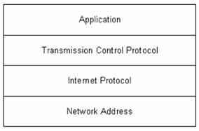
Figure 1.1 The
four-layer TCP/IP model.
Figure 1.2 An IP
packet.
During an analysis session, or sniffer
capture, it is necessary to differentiate between different types of
packet captures. The following describes the IP packet and the 14 fields
therein, as illustrated in Figure 1.2.
Version. The IP version currently
used.
IP Header Length (Length). The
datagram header length in 32-bit words.
Type-of-Service (ToS). How the
upper-layer protocol (the layer immediately above, such as transport
protocols like TCP and UDP) intends to handle the current datagram and
assign a level of importance.
Total Length. The length, in
bytes, of the entire IP packet.
Identification. An integer used to
help piece together datagram fragments.
Flag. A 3-bit field, where the
first bit specifies whether the packet can be fragmented. The second bit
indicates whether the packet is the last fragment in a series. The final
bit is not used at this time.
Fragment Offset. The location of
the fragment’s data, relative to the opening data in the original
datagram. This allows for proper reconstruction of the original
datagram.
Time-to-Live (TTL). A counter that
decrements to zero to keep packets from endlessly looping. At the zero
mark, the packet is dropped.
Protocol. Indicates the
upper-layer protocol receiving the incoming packets.
Header Checksum. Ensures the
integrity of the IP header.
Source Address/Destination Address.
The sending and receiving nodes (station, server, and/or router).
Options. Typically, contains
security options.
Data. Upper-layer information.
Key fields to note include the Source Address, Destination Address,
Options, and Data.
Now let’s look at actual sniffer
snapshots of IP Headers in Figures 1.3a and 1.3b to compare with the
fields in the previous figure.
Figure 1.3a
Extracted during the transmission of an
Internet Control Message Protocol (ICMP) ping test (ICMP is explained
later in this chapter).
 Figure
1.3b
Figure
1.3b
Extracted during the transmission of a
NetBIOS User Datagram Protocol (UDP) session request (these protocols
are described later in this chapter and in Chapter 2).
IP
Datagrams, Encapsulation, Size, and Fragmentation
IP datagrams are the very basic, or
fundamental, transfer unit of the Internet. An IP datagram is the unit
of data commuted between IP modules. IP datagrams have headers with
fields that provide routing information used by infrastructure equipment
such as routers (see Figure 1.4).
Figure 1.4 An IP datagram.
Be aware that the data in a packet is not
really a concern for the IP. Instead, IP is concerned with the control
information as it pertains to the upper-layer protocol. This information
is stored in the IP header, which tries to deliver the datagram to its
destination on the local network or over the Internet. To understand
this relationship, think of IP as the method and the datagram as the
means.
The IP header is the primary field for
gathering information, as well as for gaining control.
It is important to understand the methods
a datagram uses to travel across networks. To sufficiently travel across
the Internet, over physical media, we want some guarantee that each
datagram travels in a physical frame. The process of a datagram
traveling across media in a frame is called encapsulation. Now, let’s
take a look at an actual traveling datagram scenario to further explain
these traveling datagram methods (see Figure 1.5). This example includes
corporate connectivity between three branch offices, over the Internet,
linking Ethernet, Token Ring, and FDDI (Fiber Distributed Data
Interface) or fiber redundant Token Ring networks.
 Figure
1.5 Real-world example of a traveling datagram.
Figure
1.5 Real-world example of a traveling datagram.
An ideal situation is one where an entire
IP datagram fits into a frame; and the network it is traveling across
supports that particular transfer size. But as we all know ideal
situations are rare. One problem with our traveling datagram is that
networks enforce a maximum transfer unit (MTU) size, or limit, on the
size of transfer. To further confuse the issue, different types of
networks enforce their own MTU; for example, Ethernet has an MTU of
1500, FDDI uses 4470 MTU, and so on. When datagrams traveling in frames
cross network types with different specified size limits, routers must
sometimes divide the datagram to accommodate a smaller MTU. This process
is called fragmentation.
Routers
provide the fragmentation process of datagrams, and as such, become
vulnerable to passive and intrusive attacks.
IP Addresses, Classes, Subnet Masks
Communicating on the Internet would be almost impossible if a system of
unique addressing were not used. To prevent the use of duplicate
addresses, routing between nodes is based on addresses assigned from a
pool of classes, or range of available addresses, from the InterNetwork
Information Center (InterNIC). InterNIC assigns and controls all network
addresses used over the Internet by assigning addresses in three classes
(A, B, and C), which consist of 32-bit numbers. By default, the usable
bits for Classes A, B, and C are 8, 16, and 24 respectively. Addresses
from this pool have been assigned and utilized since the 1970s, and they
include the ranges shown in Figure 1.6; an example of an IP address is
shown in Figure 1.7.
Figure 1.6 IP address chart by class.
Figure 1.7 IP address example with
four octets.
The first octet (206) indicates a Class C
(Internet-assigned) IP address range with the format
Network.Network.Network.Host with a standard mask binary indicating
255.255.255.0. This means that we have 8 bits in the last octet for
hosts. The 8 bits that make up the last, or fourth, octet are understood
by infrastructure equipment such as routers and software in the
following manner:

In this example of a full Class C, we
only have 254 usable IP addresses for hosts; 0 and 255 cannot be used as
host addresses because the network number is 0 and the broadcast address
is 255. With the abundant utilization of Class B address space and the
flooding of requested Class C addresses, a Classless Interdomain Routing
(CIR) system was introduced in the early 1990s. Basically, a route is no
longer an IP address; a route is now an IP address and mask, allowing us
to break a network into subnets and supernets. This also drastically
reduces the size of Internet routing tables.
It is important to understand IP address masking and subnetting for
performing a security analysis, penetration hacking, and spoofing.
There’s more information on these topics later in this chapter.
Subnetting,
VLSM, and Unraveling IP the Easy Way
Subnetting is the process of dividing an
assigned or derived address class into smaller, individual, but related,
physical networks. Variable-length subnet masking (VLSM) is the
broadcasting of subnet information through routing protocols (covered in
the next chapter). A subnet mask is a 32-bit number that determines the
network split of IP addresses on the bit level.
 Figure
1.8
Real-world IP network example.
Figure
1.8
Real-world IP network example.
Example 1 Let’s take a look at a
real-world scenario of allocating IP addresses for a routed network
(Figure 1.8).
Given: 206.0.125.0 (NIC assigned Class
C). In this scenario, we need to divide our Class C address block to
accommodate three usable subnets (for offices A, B, and C) and two
subnets for future growth. Each subnet or network must have at least 25
available node addresses. This process can be divided into five steps.
Step 1 Four host addresses will be
required for each of the office’s router interfaces: Router 1 Ethernet
0, Router 2 Ethernet 0/Ethernet 1, and Router 3 Token Ring 0 (see Figure
1.9).
Step 2 Only one option will
support our scenario of five subnets with at least 25 IP addresses per
network (as shown in the Class C subnet chart in Figure 1.10).
 Figure
1.9
Real-world network example interface requirement chart.
Figure
1.9
Real-world network example interface requirement chart.

Figure 1.10 Class C subnet chart
by number of subnets versus number of hosts per subnet.
Bits in Subnet Mask: Keeping in mind the
information given earlier, let’s further explore the subnet mask bit
breakdown. When a bit is used, we indicate this with a 1:
 Number
of Subnets: Remember, in this scenario we need to divide our Class C
address block to accommodate three usable subnets (for offices A, B, and
C) and two subnets for future growth with at least 25 available node
addresses per each of the five networks.
Number
of Subnets: Remember, in this scenario we need to divide our Class C
address block to accommodate three usable subnets (for offices A, B, and
C) and two subnets for future growth with at least 25 available node
addresses per each of the five networks.
To make this process as simple as
possible, let’s start with the smaller number—that is, 5 for the
required subnets or networks, as opposed to 25 for the available nodes
needed per network. To solve for the required subnets in Figure 1.9),
we’ll start with the following equation, where we’ll solve for n in 2n –
2, being sure to cover the required five subnets or networks.
Let’s start with the power of 2 and work
our way up:
22 – 2 = 2 23 – 2 = 6 24 – 2 = 14
The (3rd power) in the equation indicates
the number of bits in the subnet mask. Here we see that 23 – 2 = 6
subnets if we use these 3 bits. This will cover the required five
subnets with an additional subnet (or network) left over.
Number of Hosts per Subnet: Now let’s
determine the number of bits left over for available host addresses. In
this scenario, we will be using 3 bits in the mask for subnetting. How
many are left over?
Out of the given 32 bits that make up IP
addresses, the default availability (for networks versus hosts), as
previously explained, for Classes A, B, and C blocks are as follows:
Class A: 8 bits
Class B: 16 bits
Class C: 24 bits
Our scenario involves a Class C block
assigned by InterNIC. If we subtract our default bit availability for
Class C of 24 bits (as shown) from the standard 32 bits that make up IP
addresses, we have 8 bits remaining for networks versus hosts for Class
C blocks.
Next, we subtract our 3 bits used for
subnetting from the total 8 bits remaining for network versus hosts,
which gives us 5 bits left for actual host addressing:
Let’s solve an equation to see if 5 bits
are enough to cover the required available node addresses of at least 25
per subnet or network:
25 – 2 = 30
Placing the remaining 5 bits back into
our equation gives us the available node addresses per subnet or
network, 25 – 2 = 30 host addresses per six subnets or networks
(remember, we have an additional subnet left over).
From these steps, we can divide our Class
C block using 3 bits to give us six subnets with 30 host addresses each.
Step 3
Now that we have determined the subnet
mask, in this case 255.255.255.224 (3 bits), we need to calculate the
actual network numbers or range of IP addresses in each network. An easy
way to accomplish this is by setting the host bits to 0. Remember, we
have 5 bits left for hosts:
With the 5 host bits set to 0, we set the
first 3 bits to 1 in every variation, then calculate the value (for a
shortcut, take the first subnet value=32 and add it in succession to
reveal all six subnets):
Now let’s take a look at the network
numbers of our subnetted Class C block with mask 255.255.255.224:
Step 4
Now that we have solved the network
numbers, let’s resolve each network’s broadcast address by setting host
bits to all 1s. The broadcast address is defined as the system that
copies and delivers a single packet to all addresses on the network. All
hosts attached to a network can be notified by sending a packet to a
common address known as the broadcast address:
Let’s take a look at the network
broadcast addresses of our subnetted Class C block with mask
255.255.255.224:
Step 5
So what are the available IP addresses
for each of our six networks anyway? They are the addresses between the
network and broadcast addresses for each subnet or network (see Figure
1.11).
 Figure
1.11
Figure
1.11
Available IP addresses for our networks.
Unraveling IP with Shortcuts
Let’s take a brief look at a shortcut for
determining a network address, given an IP address. Given: 206.0.139.81
255.255.255.224. To calculate the network address for this host, let’s
map out the host octet (.81) and the subnet-masked octet (.224) by
starting from the left, or largest, number:
Now we can perform a mathematic “logical
AND” to obtain the network address of this host (the value 64 is the
only common bit):
We simply put the 1s together
horizontally, and record the common value (205.0.125.64).
ARP/RARP Engineering: Introduction to Physical Hardware Address Mapping
Now that we have unearthed IP addresses
and their 32-bit addresses, packet/datagram flow and subnetting, we need
to discover how a host station or infrastructure equipment, such as a
router, match an IP address to a physical hardware address. This section
explains the mapping process that makes communication possible. Every
interface, or network interface card (NIC), in a station, server, or
infrastructure equipment has a unique physical address that is
programmed by and bound internally by the manufacturer. One goal of
infrastructure software is to communicate using an assigned IP or
Internet address, while hiding the unique physical address of the
hardware. Underneath all of this is the address mapping of the assigned
address to the actual physical hardware address. To map these addresses,
programmers use the Address Resolution Protocol (ARP). Basically, ARP is
a packet that is broadcasted to all hosts attached to a physical
network. This packet contains the IP address of the node or station with
which the sender wants to communicate. Other hosts on the network ignore
this packet after storing a copy of the sender’s IP/hardware address
mapping. The target host, however, will reply with its hardware address,
which will be returned to the sender, to be stored in its ARP response
cache. In this way, communication between these two nodes can ensue (see
Figure 1.12).
The hardware address is usually hidden by
software, and therefore can be defined as the ultimate signature or
calling card for an interface.
 Figure
1.12 ARP resolution.
Figure
1.12 ARP resolution.
ARP Encapsulation and Header
Formatting
It is important to know that ARP is not
an Internet protocol; moreover, ARP does not leave the local logical
network, and therefore does not need to be routed. Rather, ARP must be
broadcasted, whereby it communicates with every host interface on the
network, traveling from machine to machine encapsulated in Ethernet
packets (in the data portion).
Figure 1.13 An ARP/RARP packet.
illustrates the encapsulation of an ARP
packet including the Reverse Address Resolution Protocol (RARP) (which
is discussed in the next section). The packet components are defined in
the following list
RARP Transactions, Encapsulation
The Reverse Address Resolution Protocol
(RARP), to some degree, is the opposite of ARP. Basically, RARP allows a
station to broadcast its hardware address, expecting a server daemon to
respond with an available IP address for the station to use. Diskless
machines use RARP to obtain IP addresses from RARP servers. It is
important to know that RARP messages, like ARP, are encapsulated in
Ethernet frames (see Figure 1.14, Excerpt from Figure 1.13). Likewise,
RARP is broadcast from machine to machine, communicating with every host
interface on the network.
 RARP
Service
RARP
Service
The RARP Daemon (RARPd) is a service that
responds to RARP requests. Diskless systems typically use RARP at boot
time to discover their 32-bit IP address, given their 48-bit hardware
Ethernet address. The booting machine sends its Ethernet address,
encapsulated in a frame as a RARP request message. The server running
RARPd must have the machine’s name-to-IP-address entry, or it must be
available from the Domain Name Server (DNS) with its
name-to-Ethernet-address. With these sources available, the RARPd server
maps this Ethernet address with the corresponding IP address.
Transmission Control Protocol
IP has many weaknesses, one of which is
unreliable packet delivery—packets may be dropped due to transmission
errors, bad routes, and/or throughput degradation. The Transmission
Control Protocol (TCP) helps reconcile these issues by providing
reliable, stream-oriented connections. In fact,
TCP/IP is predominantly based on TCP
functionality, which is based on IP, to make up the TCP/IP suite. These
features describe a connection-oriented process of communication
establishment. There are many components that result in TCP’s reliable
service delivery. Following are some of the main points:
Streams. Data is systematized and
transferred as a stream of bits, organized into 8-bit octets or bytes.
As these bits are received, they are passed on in the same manner.
Buffer Flow Control. As data is passed in
streams, protocol software may divide the stream to fill specific buffer
sizes. TCP manages this process, and assures avoidance of a buffer
overflow. During this process, fast-sending stations may be stopped
periodically to keep up with slow-receiving stations.
Virtual Circuits. When one station
requests communication with another, both stations inform their
application programs, and agree to communicate. If the link or
communications between these stations fail, both stations are made aware
of the breakdown and inform their respective software applications. In
this case, a coordinated retry is attempted.
Full Duplex Connectivity. Stream transfer
occurs in both directions, simultaneously, to reduce overall network
traffic.
 Figure
1.15 TCP windowing example.
Figure
1.15 TCP windowing example.
Sequencing and Windowing
TCP organizes and counts bytes in the
data stream using a 32-bit sequence number. Every TCP packet contains a
starting sequence number (first byte) and an acknowledgment number (last
byte). A concept known as a sliding window is implemented to make stream
transmissions more efficient. The sliding window uses bandwidth more
effectively, because it will allow the transmission of multiple packets
before an acknowledgment is required. Figure 1.15 is a real-world
example of the TCP sliding window. In this example, a sender has bytes
to send in sequence (1 to 8) to a receiving station with a window size
of 4. The sending station places the first 4 bytes in a window and sends
them, then waits for an acknowledgment (ACK=5). This acknowledgment
specifies that the first 4 bytes were received. Then, assuming its
window size is still 4 and that it is also waiting for the next byte
(byte 5), the sending station moves the sliding window 4 bytes to the
right, and sends bytes 5 to 8. Upon receiving these bytes, the receiving
station sends an acknowledgment (ACK=9), indicating it is waiting for
byte 9. And the process continues. At any point, the receiver may
indicate a window size of 0, in which case the sender will not send any
more bytes until the window size is greater. A typical cause for this
occurring is a buffer overflow.
TCP Packet Format and
Header Snapshots
Keeping in mind that it is important to
differentiate between captured packets—whether they are TCP, UDP, ARP,
and so on—take a look at the TCP packet format in Figure 1.16, whose
components are defined in the following list:
Figure 1.16 A TCP packet.
Ports, Endpoints,
Connection Establishment
TCP enables simultaneous communication
between different application programs on a single machine. TCP uses
port numbers to distinguish each of the receiving station’s
destinations. A pair of endpoints identifies the connection between the
two stations, as mentioned earlier. Colloquially, these endpoints are
defined as the connection between the two stations’ applications as they
communicate; they are defined by TCP as a pair of integers in this
format: (host, port). The host is the station’s IP address, and port is
the TCP port number on that station. An example of a station’s endpoint
is: 206.0.125.81:1026 (host)(port) An example of two stations’ endpoints
during communication is:
This technology is very important in TCP,
as it allows simultaneous communications by assigning separate ports for
each station connection. When a connection is established between two
nodes during a TCP session, a three-way handshake is used. This process
starts with a one-node TCP request by a SYN/ACK bit, and the second node
TCP response with a SYN/ACK bit. At this point, as described previously,
communication between the two nodes will proceed. When there is no more
data to send, a TCP node may send a FIN bit, indicating a close control
signal. At this intersection, both nodes will close simultaneously.
Figure 1.17a Extracted from an
HTTP Internet Web server transmission.
 Figure
1.17b Extracted from a sliding window sequence
transmission.
Figure
1.17b Extracted from a sliding window sequence
transmission.
User Datagram Protocol
The User Datagram Protocol (UDP) operates
in a connectionless fashion; that is, it provides the same unreliable,
datagram delivery service as IP. Unlike TCP, UDP does not send SYN/ACK
bits to assure delivery and reliability of transmissions. Moreover, UDP
does not include flow control or error recovery functionality.
Consequently, UDP messages can be lost, duplicated, or arrive in the
wrong order. And because UDP contains smaller headers, it expends less
network throughput than TCP and so can arrive faster than the receiving
station can process them. UDP is typically utilized where higher-layer
protocols provide necessary error recovery and flow control. Popular
server daemons that employ UDP include Network File System (NFS), Simple
Network Management Protocol (SNMP), Trivial File Transfer Protocol
(TFTP), and Domain Name System (DNS), to name a few.
UDP Formatting, Encapsulation, and Header
Snapshots
UDP messages are called user datagrams.
These datagrams are encapsulated in IP, including the UDP header and
data, as it travels across the Internet. Basically, UDP adds a header to
the data that a user sends, and passes it along to IP. The IP layer then
adds a header to what it receives from UDP. Finally, the network
interface layer inserts the datagram in a frame before sending it from
one machine to another. As just mentioned, UDP messages contain smaller
headers and consume fewer overheads than TCP. The UDP datagram format is
shown in Figure 1.18, and its components are defined in the following
list.
Multiplexing, Demultiplexing, and Port Connections
UDP provides multiplexing (the method for
multiple signals to be transmitted concurrently into an input stream,
across a single physical channel) and demultiplexing (the actual
separation of the streams that have been multiplexed into a common
stream back into multiple output streams) between protocol and
application software. Multiplexing and demultiplexing, as they pertain
to UDP, transpire through ports. Each station application must negotiate
a port number before sending a UDP datagram. When UDP is on the
receiving side of a datagram, it checks the header (destination port
field) to determine whether it matches one of station’s ports currently
in use. If the port is in use by a listening application, the
transmission proceeds; if the port is not in use, an ICMP error message
is generated, and the datagram is discarded.
Figure 1.19 Extracted after the IP
portion of a domain name resolution from a DNS request transmission
Internet Control Message Protocol
The Internet Control Message Protocol
(ICMP) delivers message packets, reporting errors and other pertinent
information to the sending station or source. Hosts and infrastructure
equipment use this mechanism to communicate control and error
information, as they pertain to IP packet processing.
ICMP Format,
Encapsulation, and Delivery
ICMP message encapsulation is a two-fold
process. The messages are encapsulated in IP datagrams, which are
encapsulated in frames, as they travel across the Internet. Basically,
ICMP uses the same unreliable means of communications as a datagram.
This means that ICMP error messages may be lost or duplicated. The ICMP
format includes a message type field, indicating the type of message; a
code field that includes detailed information about the type; and a
checksum field, which provides the same functionality as IP’s checksum
(see Figure 1.20). When an ICMP message reports an error, it includes
the header and data of the datagram that caused the specified problem.
This helps the receiving station to understand which application and
protocol sent the datagram. (The next section has more information on
ICMP message types.)

Figure 1.20 Illustration of an ICMP
datagram.
Figure 1.21 ICMP message chart.
ICMP Messages, Subnet Mask Retrieval
There are many types of useful ICMP
messages; Figure 1.21 contains a list of several, which are described in
the following list. Echo Reply (Type 0)/Echo Request (Type 8). The basic
mechanism for testing possible communication between two nodes. The
receiving station, if available, is asked to reply to the ping. An
example of a ping is as follows:
STEP 1:
BEGIN ECHO REQUEST Ping 206.0.125.81 (at
the command prompt)
Reply from 206.0.125.81: bytes-32
time<10ms TTL=128 (from receiving station 206.0.125.81)
Reply from 206.0.125.81: bytes-32
time<10ms TTL=128
Reply from 206.0.125.81: bytes-32
time<10ms TTL=128
Reply from 206.0.125.81: bytes-32
time<10ms TTL=128
Destination Unreachable (Type 3).
There are several issuances for this message type, including when a
router or gateway does not know how to reach the destination, when a
protocol or application is not active, when a datagram specifies an
unstable route, or when a router must fragment the size of a datagram
and cannot because the Don’t Fragment Flag is set. An example of a Type
3 message is as follows:
STEP 1: BEGIN ECHO REQUEST Ping
206.0.125.81 (at the command prompt)
STEP 2: BEGIN ECHO REPLY Pinging
206.0.125.81 with 32 bytes of data:
Destination host unreachable.
Source Quench (Type 4). A basic
form of flow control for datagram delivery. When datagrams arrive too
quickly at a receiving station to process, the datagrams are discarded.
During this process, for every datagram that has been dropped, an ICMP
Type 4 message is passed along to the sending station. The Source Quench
messages actually become requests, to slow down the rate at which
datagrams are sent. On the flip side, Source Quench messages do not have
a reverse effect, whereas the sending station will increase the rate of
transmission.
Route Redirect (Type 5). Routing
information is exchanged periodically to accommodate network changes and
to keep routing tables up to date. When a router identifies a host that
is using a nonoptional route, the router sends an ICMP Type 5 message
while forwarding the datagram to the destination network. As a result,
routers can send Type 5 messages only to hosts directly connected to
their networks.
Datagram Time Exceeded (Type 11).
A gateway or router will emit a Type 11 message if it is forced to drop
a datagram because the TTL (Time-to-Live) field is set to 0. Basically,
if the router detects the TTL=0 when intercepting a datagram, it is
forced to discard that datagram and send an ICMP message Type 11.
Datagram Parameter Problem (Type 12).
Specifies a problem with the datagram header that is impeding further
processing. The datagram will be discarded, and a Type 12 message will
be transmitted.
Timestamp Request (Type 13)/Timestamp
Reply (Type 14). These provide a means for delay tabulation of the
network. The sending station injects a send timestamp (the time the
message was sent) and the receiving station will append a receive
timestamp to compute an estimated delay time and assist in their
internal clock synchronization.
Figure 1.22 ICMP header sniffer
capture.
Information Request (Type
15)/Information Reply (Type 16). As an alternative to RARP
(described previously), stations use Type 15 and Type 16 to obtain an
Internet address for a network to which they are attached. The sending
station will emit the message, with the network portion of the Internet
address, and wait for a response, with the host portion (its IP address)
filled in.
Address Mask Request (Type 17)/Address
Mask Reply (Type 18). Similar to an Information Request/Reply,
stations can send Type 17 and Type 18 messages to obtain the subnet mask
of the network to which they are attached. Stations may submit this
request to a known node, such as a gateway or router, or broadcast the
request to the network.
ICMP Header Snapshots
Figure 1.22 on page 35 contains snapshots
of an ICMP Header. The first was extracted after the IP portion of an
ICMP ping test transmission; the second was extracted during an
unreachable ping test.
Wanna Make some money?
If
you have access to your own email account, you can get paid.