chapter 2

Finite Element Method and mesh generation

The ideas that gave birth to the Finite Element Methods (FEM) evolved gradually from the independent contributions of many people in the fields of engineering, applied mathematics, and physics.

Hrenikoff (1941) found out that the elastic behavior of a physically continuous plate would be similar, under certain loading conditions, to a framework of physically separate one-dimensional rods and beams, connected together as discrete points. The problem then handled for trusses and frameworks with similar computational methods.

Courant’s (1943) paper is a classic for finite element methods. To solve the torsion problem in elasticity, he defined piecewise linear polynomials over a triangularized region. Schoenberg’s (1946) paper gave birth to the theory of splines, recommending the use of piecewise polynomials for approximation and interpolation. Synge (1957) used piecewise linear functions defined over triangularized region with a Reitz variational procedure.

With the introduction of high-speed digital computers, Langefors (1952) and Argyris (1954) took the framework analysis procedures and reformulated them into a matrix format suited for efficient automatic computation. McMahon (1953) solved a three-dimensional electrostatic problem using tetrahedral elements and linear trial functions. Polya (1954), Hersh (1955), and Weinberger (1956) used ideas similar to Courant’s to estimate bounds for eigenvalues.

Turner et al. (1956) modeled the odd-shaped wing panels of high-speed aircraft as an assemblage of smaller panels of simple triangular shape. This was a breakthrough as it made it possible to model two- or three-dimensional structures as assemblages of similar two- or three-dimensional pieces rather than of one-dimensional bars. Greenstadt (1959) divided a domain into cells, assigned a different function to each cell, and applied a variational principle. White (1962) and Friedrichs (1962) used triangular elements to develop difference equations from variational principles. The name of the method, “finite elements”, first appeared in Clough’s  (1960) paper. Melosh (1963), Besseling (1963), Jones(1964), and Fraeijs de Veubeke (1964) showed that the FEM could be identified as a form of the Ritz variational method using piecewise-defined trial functions. Zienkiewicz & Cheung (1965) showed that FEM is applicable to all field problems that could be placed in variational form.

 In order to better conform to curve boundaries, curved finite elements have been widely used in recent years (Ertürk, 1995). Such elements are called the ”isoparametric” elements (Zienkiewicz, 1971). Irregular computational grids have become increasingly popular for a wide variety of numerical modeling applications as they allow points to be situated on curved boundaries of irregularly shaped domains.

2.1.            Basics of Finite Element Methods

FEM is a numerical technique for finding an approximate numerical solution to the governing equations of a problem. FEM is applicable to solid mechanics, heat transfer, fluid mechanics, acoustics, electro-magnetism and quantum mechanics problems. Those problems can be described by differential, integral or variational equations; they can be boundary-value, eigen-value or initial-value problems. The domain of the problem may be a complicated or a simple geometry. Physical properties (density, conductivity, etc.) may vary throughout the domain. Boundary conditions or initial conditions can be given in many different forms (Burnett, 1987).

For most practical problems, it is impossible to find an explicit expression for the unknown, in terms of known functions, which exactly satisfies the governing equations and the boundary conditions. The purpose of the FEM is to find an explicit expression for the unknown, in terms of known functions, which approximately satisfies the governing equations and the boundary conditions (the approximate solution may satisfy some of the boundary conditions exactly).

FEM uses a trial-solution approach in order to obtain an approximate solution. The trial-solution approach has three major steps:

·        Start with an approximate solution for the unknown

·        Apply an optimizing criterion to the approximate solution

·        Estimate the accuracy of the approximate solution

There are two major types of optimizing criteria, which can be applied to the approximate solution:

·        Methods of Weighted Residuals (MWR), which is used when the governing equations are differential equations (Canuto et al., 1988).

·        Ritz Variational Method (RVM), which is used when governing equations are variational (integral) equations (Krasnov et al., 1975 and Mura and Koya, 1992).

MWR criteria try to minimize an expression of error in the differential equation, while RVM try to minimize some physical quantity, such as energy.  Some of the most popular MWR criteria are collocation method, sub-domain method, least-squares method and Galerkin Method. The FE model adopted in this study, ADAM model (see Chapter 3), uses the Galerkin method as an optimizing criterion.

Accuracy can be defined as the closeness of the approximate solution to the exact solution. If the estimate of accuracy is not in an acceptable range then the trial solution will be constructed again and the same procedure will be applied until an acceptable accuracy is reached.

First step in applying FEM to a system is to divide the domain into rectangular or triangular elements. In the next section, the procedure adopted in this study for generating a mesh in the Great Bay Estuary is explained.

2.2.            Mesh Generation in the Great Bay Estuary System

In order to use ADAM model (see next chapter for detail), a mesh defining the system of interest with triangular elements is needed. A public domain search for mesh generation software uncovers two results:

·        MESHTOOLS developed for MATLAB by Tom Gross from Skidaway Institute of Oceanography, Savannah, Georgia and

·        TRIANGLE developed by Jonathan Richard Shewchuk from the Carnegie Mellon University, Pittsburgh, Pennsylvania as a part of the parallel FEM tools generation project Archimedes.

License and version problems in MATLAB and lack of documentation for MESHTOOLS directed us to use TRIANGLE for the present purpose. TRIANGLE is well documented, capable of doing all the calculations and refinements needed for mesh generation and is proven to work correctly. All the meshes generated in this study were created using TRIANGLE (see http://www.cs.cmu.edu/~quake/triangle.html).

2.2.1.      FE Mesh Generation Tool, TRIANGLE

Basic finite element mesh generation is almost a standard procedure. It consists of a Delaunay triangulation routine complemented with refinement and interpolation routines. A Delaunay triangulation of a point set is a triangulation of the point set with the property that no point in the point set falls in the interior of the circumcircle (circle that passes through all three vertices) of any triangle in the triangulation. The circumcircle of a triangle is the unique circle that passes through all three vertices of the triangle (Shewchuk,1996).

A triangle is said to be bad if it has an angle too small or an area too large to satisfy the user's constraints. A bad triangle is split by inserting a vertex at its circumcenter (the center of its circumcircle); the Delaunay property guarantees that the triangle is eliminated.

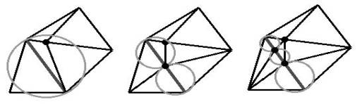
Figure 2-1. Each bad triangle is split by inserting a vertex at its circumcenter and maintaining the Delaunay property.

TRIANGLE can generate meshes in two different ways. The first one is by reading a PSLG file with an extension (.poly), which can specify points, segments (shorelines), holes (islands), and regional attributes and area constraints. A Planar Straight Line Graph (PSLG) is a collection of points and segments. Segments are simply edges whose endpoints are points in the PSLG. The second way is by reading a standard node and an element connectivity file. The node files have an extension (.node) and the element files have an extension (.ele). In this study, a PSLG file was used to generate the initial mesh. TRIANGLE generates exact Delaunay triangulations, constrained Delaunay triangulations and conforming Delanuay triangulations.

A constrained Delaunay triangulation of a PSLG is similar to a Delaunay triangulation but each PSLG segment is present as a single edge in the triangulation. A conforming Delaunay triangulation of a PSLG is a true Delaunay triangulation in which each PSLG segment may have been subdivided into several edges by the insertion of additional points. These inserted points are necessary to allow the segments to exist in the mesh while maintaining the Delaunay property.

Conforming Delaunay triangulation of a PSLG can be generated with no small angles and are thus suitable for finite element analysis. TRIANGLE is capable of refining already existing meshes by imposing maximum triangle areas or by defining minimum element angles. In this way, attributes belonging to each node are also interpolated.

2.2.2.      Extracting Data for the Mesh Generation

The first step in creating a FE mesh for Great Bay Estuary system is to define the shoreline boundary. The mean high water (MHW) level as it appears on USGS 1:25000 metric 7.5-minute topographic charts is used for this purpose. Second step is to identify the open boundaries at the mouth of the estuary and at the upriver ends of the rivers that empty into the Great Bay. A straight line going from Kittery Point to the Odiornes Point on Newcastle Island is used as the open boundary. The dams on the rivers as identified on the USGS charts are used as upper open boundaries. Third step is to identify all the island MHW shorelines in the estuary system. They are input as holes into the mesh generation program, TRIANGLE. Then some of the islands are regrouped and eliminated. The very small islands are eliminated, while some very close ones are connected together. After this procedure, the number of islands is decreased from 62 to 21. It is presumed that these improvements will have no significant effect on the results since they are not to interfere with the main estuary circulation at a high rate.

The coordinates of all the boundaries are extracted from UNH Jere A. Chase Ocean Engineering Laboratory archives, which are in Arc/Info GIS (Geographical Information System) format. The NAD83 (North American 1983 Datum) is used to convert these coordinates to New Hampshire State Plane Coordinate System, which has its origin at Universal Transverse Mercator, Zone 19. This conversion from latitude longitude format to meters is necessary for finite element modeling purposes. The finite element nodes with known depths are entered into the improved Arc/Info maps by digitizing them from NOAA nautical charts. The NOAA charts are mainly prepared for navigational purposes and give the depths in feet at mean lower low water.

Bathymetry resolution is the main problem. The bathymetric depths have to be interpolated from the data that is available. There is a lack of detail in depth readings especially between Piscataqua River Bridge and the Railroad Bridge in Piscataqua River. At a later stage, more bathymetry data is taken throughout the Great Bay Estuary by Ata Bilgili (graduate student at Jere A. Chase OEL) and is blended with the existing data.

2.2.3.      Preliminary Meshes for the Great Bay Estuary System

The extracted boundary and node coordinates are converted to a format that can be used with TRIANGLE.  The mesh is improved by refining the boundaries where large amounts of very small elements are clustered. The mesh is refined using TRIANGLE with a minimum angle of 30° restriction in order to avoid possible numerical instabilities with any finite element model in the future. The “GBEST1” mesh is created to model the whole estuary system with our best available bathymetric data. GBEST1 mesh has 26455 nodes and 46740 elements. Since it exceeds the computational limitation in the beginning, the "divide and conquer" strategy is adopted.

Considerable effort is put in modeling the entire Great Bay Estuary System with ADAM model.  The mesh is subdivided into small enough sections to simulate individual rivers and smaller regions of interest, with the final goal of simulating the whole Great Bay Estuary System including only the essential components in order to fit the computational limitation.  This strategy enables us to gain valuable experience on the limitation of ADAM software in modeling the realistic features and processes occurring in the domain, and the importance of each sub-domain contribution to the entire estuary system.  Detailed simulation results of each component of the estuary system and a vast combination of the important components are obtained.  Results include mass conservation, residual current, transports, bottom stress, and sediment transport at dynamical equilibrium, time series of the non-linear asymmetric flood and ebb cycle as M₂ tidal forcing is applied at the appropriate open boundaries with predicted elevation data from Swift and Brown (1983). Most of the

simulation results are presented at:                                                                                                                                                               http://nemo.unh.edu/safak/introduction.html

The sub-domains include the following meshes (see Table 2-1.):

·        BR5:   models the Bellamy River.

·        YR5:   models the Oyster River.

·        port3: models the waterway between the Portsmouth Harbor and the Lower  Piscataqua River.   

·        gbay6: models the Great Bay area including the Great Bay, the Little Bay,   the Squamscott River, the Winnicut River, and the Lamprey River.

·        pby:   models the Bellamy, the Piscataqua and the Oyster Rivers.

·        pr6:   models the Lower and the Upper Piscataqua River.

·        gbriv: models the Great Bay, the Little Bay with the Oyster and the  Bellamy Rivers.

·        phriv: models the Portsmouth Harbor section and the Lower and the Upper Piscataqua Rivers.

 

Table 2- 1. Numeric and geomorphologic properties of the preliminary meshes used during the modeling efforts for the Great Bay Estuary system.  All the coordinates are given in New Hampshire State Plane coordinate system (NAD83).

	Numeric Properties			Geomorphologic Properties
Mesh Name	Number of nodes (NN)	Number of Elements (NE)	Band width (BW)	Horizontal coordinate (m)	Bathymetry Range (m)
BR5	1054	1828	49
YR5	1409	2415	63
port3	8577	14974	243
gbay6	10439	18526	211
pby	8621	15404	173
pr6	3417	6043	79
gbriv	10223	18710	199
phriv	12113	21235	243

 

.

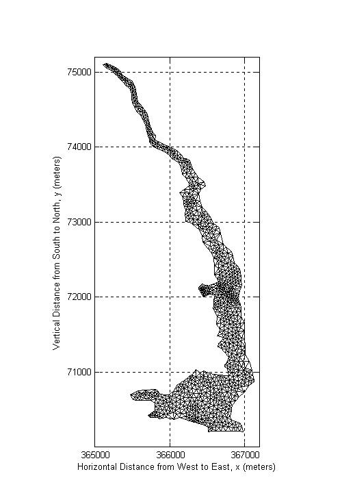
Figure 2-2. Bellamy River (BR5) mesh has 1054 nodes and 1828 triangular elements. Maximum depth value in this section is 7.1m.

 

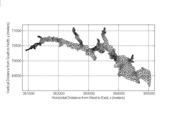
Figure 2-3. Oyster River (YR5) mesh has 1409 nodes and 2415 elements. Maximum depth value in this section is 8.79m.

 

 

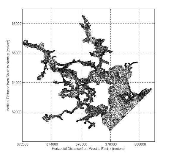
Figure 2-4. Portsmouth Harbor (port3) mesh has 8577 nodes and 14974 elements. Maximum depth value in this section is 25.4m.

 

 

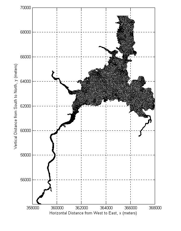
Figure 2-5. Great Bay (gbay6) mesh has 10439 nodes and 18526 elements. Maximum depth value in this section is 21.8m.

 

 

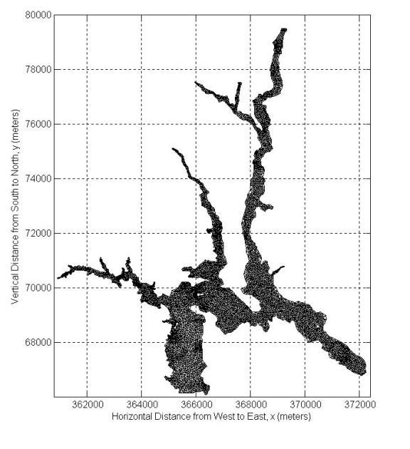
Figure 2-6. Three River (pby) mesh has 8621 nodes and 15404 elements. Maximum depth value in this section is 23.0m.

 

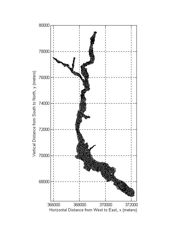
Figure 2-7. Piscataqua River (pr6) mesh 3417 nodes and 6043 elements. Maximum depth value in this section is 18.93m.

 

 

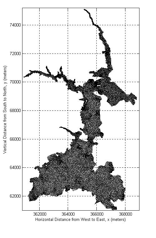
Figure 2-8. Great Bay  (gbriv) mesh with the Oyster and Bellamy rivers has 10223 nodes and 18710 elements. Maximum depth value in this section is 23.0m.

 

Figure 2-9. Portsmouth Harbor and Piscataqua River (phriv) mesh has 12113 nodes and 21235 elements. Maximum depth value in this section is 25.4m.

 

 

All the above-mentioned meshes are then merged and some small tributaries are cut and the GBES4 mesh is obtained. GBES4 is the master mesh, which is used for simulating the whole estuary.  The master mesh is cut into pieces when needed for individual purposes.

The bathymetry in the channels in Great Bay area is then fine-tuned with the data obtained through personal communications with Dr. Fred Short at Jackson Estuarine Laboratory.  The mesh with the detailed bathymetry in the Great Bay section is called the “gbay18” mesh. The details of this mesh with the bathymetry contours are shown in Figure 2-10.

 

Figure 2-10. Bathymetry contours and the final mesh detail of the gbes18 mesh.