CHAPTER 5

tides and tidal forcing

 Gravitational attraction of the sun and the moon are responsible for the tidal motions on the earth. Tides are caused by the movement of the sun and the moon relative to points on the earth’s surface. Gravitational force is proportional to the product of the masses of the two objects and inversely proportional to the square of the distance between them. The mass of the sun is about  times that of the moon. The distance between the sun and the earth is 400 times longer than the distance between the moon and the earth. Thus, tidal forces produced by the moon are slightly more than twice those of the sun (Knauss, 1997).

The tides in the global oceans cause the rhythmic rise and fall of sea level along the world’s coastlines. In some places, the sea level rises and falls with a period of about half a day (these are called semi-diurnal tides), whereas in other places the period is more like a day (called diurnal tides). In some places, the tides are mixed, with changing periods during the year, when the sun and the moon line up with the Earth.

To model tidal motions, it is necessary to prescribe the astronomical forcing. The tidal forcing term in the equations of motion can be expressed as a Fourier series, with each term representing a tidal constituent. There are many tidal constituents. Most of the tidal constituents are given in Table 5-1.

 

Table 5-1. Tidal Harmonic Components (from Knauss, 1997).

Name of Partial Tide	Symbol	Period (hrs)	Coefficient ratio M2=100
Semidiurnal components
Principal lunar	M2	12.42	100.0
Principle solar	S2	12.00	46.6
Larger lunar elliptic	N2	12.66	19.2
Lunisolar semidiurnal	K2	11.97	12.7
Larger solar elliptic	T2	12.01	2.7
Smaller lunar elliptic	L2	12.19	2.8
Lunar elliptic second order	2N2	12.91	2.5
Larger lunar evectional		12.63	3.6
Smaller lunar evectional		12.22	0.7
Variational		12.87	3.1
Diurnal components
Lunisolar diurnal	K1	23.93	58.4
Principle lunar diurnal	O1	25.82	41.5
Principle solar diurnal	P1	24.07	19.4
Larger lunar elliptic	Q1	26.87	7.9
Smaller lunar elliptic	M1	24.84	3.3
Small lunar elliptic	J1	23.10	3.3
Long –period components
Lunar fortnightly	Mf	327.67	17.2
Lunar monthly	Mm	661.30	9.1
Solar semiannual	Ssa	2191.43	8.0

 

 

In order to make tidal predictions at a location, one must have tidal records at that location. Harmonic analysis helps to determine the role of tidal constituents at the given location. Using astronomical tables, future ocean tides can be predicted at a given location.

 

5.1.            Boundary Conditions

Three different types of boundary conditions can be specified for FE model simulations:

·        Essential Boundary Condition: An equation relating the unknown value and/or of its derivatives up to order m-1, at the points on the boundary.

·        Natural Boundary Condition: An equation relating the values of any of the derivatives of the unknown value from order m to 2m-1, at points on the boundary.

·        Mixed Boundary Condition: It is a mix of the other two, containing the unknown and/or any of its derivatives up to order 2m-1.

Essential boundary conditions involve the lower-order derivatives and sometimes referred to as Dirichlet boundary conditions. Natural boundary conditions involve the higher-order derivatives and sometimes referred to as Neumann boundary conditions. The mixed boundary conditions also referred as Robin boundary condition (Burnett, 1987).

M₂, S₂ and N₂ are the most dominant constituents in the Great Bay estuary system (Swift and Brown, 1983). Throughout this study, a harmonic analysis program TIDHAR was used to make predictions for the boundary forcing at the open boundaries of each mesh. For that purpose, 1975 observational data that we had in our archives was used.

 

5.2.            Observational Data

During the summer of 1975, the University of New Hampshire (UNH) in cooperation with the National Ocean Survey (NOS) performed a comprehensive field program, designed to measure the tidal elevations and currents within the Great Bay Estuary.

UNH investigated the vertical and horizontal variability of estuarine currents and water properties at selected locations in the estuary. The purpose of the NOS survey was to update tidal elevation and current prediction data, redefine and update tidal datum planes for land movement and shoreline determination, and acquire water circulation data to be used for future ecological studies of the area.

The NOS deployed a number automatic digital recording (ADR) tidal gauges and current meters at stations shown in Figure 5-1. The ADR tide gauges recorded six-minute values of the sea level, as measured by a float in the standard NOS tidal well to a precision of better than 3 cm resolution.

 

 

 

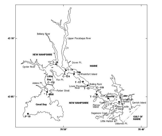
Figure 5-1. Location map of the summer 1975, NOS/UNH sea level stations (·). The transects are the ones through which Swift and Brown (1983) estimated cross-section averaged currents.

 

 

 

 

 

 

 

5.3.            Sea Level Observations

A harmonic analysis of the sea level records showed that the dominant M₂ semi-diurnal constituent amplitude decreases from 1.29m at open ocean station T-5 to 0.83m at station T-16 at the mouth of Bellamy River and increases throughout Little and Great Bays to the head of the inner estuary at station T-19 (Swift and Brown, 1983). The 70^o phase lag of the sea level at station T-19 relative to the sea level at station T-5 explains most of the corresponding 2.5-hour time lag of total sea level.

 

 

Table 5- 2. Summary of sea level data from Swenson et al. (1977)

 

 

 

 

5.4.            Current Observations

The NOS current time series are measured at the locations given in Table 5- 3 and shown in Figure 5-1. A typical mooring consists of an anchored surface floatation unit, from which a string of Savonius rotor current meters and a heavy weight are suspended to minimize the current-induced tilt of the array. The nominal depths of the current measurements used are 4.6m and 9.2m, respectively. Any data pair whose direction falls outside 15^o of the mean direction is discarded. The remaining speeds and directions are averaged. The estimated precision of the measured current speed and direction are 2.6 cm/sec and 2.5^o, respectively, for zero tilt and speeds less than 52 cm/sec. The estimated precision of speeds greater than 52 cm/sec is about 5.0 cm/sec (Swenson et al., 1977).

Swift and Brown (1983) describe how currents and sea levels were aggregated to form estuarine cross-section averaged longitudinal current time series at the above-mentioned locations. Observed cross-section averaged current is based on vertically averaged current measurements made at a single mooring at each cross-section. Two multipliers are applied to the axial component of the vertically averaged, station time series: one for the flood and one for the ebb. The multipliers are determined such that the net transport over the particular phase (flood or ebb) agrees with the cumulative tidal prism inland of the cross-section. Prism is estimated using nautical charts and average tidal ranges. The harmonic constants for the astronomical M₂, S₂, N₂, K₁, and O₁, tidal constituents, as well as the nonlinear shallow water constituents of M₄ and M₆ are determined by a harmonic analysis of these cross-section averaged current time series. The estimated uncertainty of the cross-section averaged currents is 10%.

 

Table 5- 3. Summary of current meter data from Swenson et al. (1977)