CHAPTER 3

The shallow, small-scale estuaries are non-linear. The hydrodynamics in these estuaries are well described by the classical two-dimensional shallow water equations. However, small length scales, combined with near-critical flow conditions as the depth approaches zero, makes the control of advection the dominant computational theme, even when other processes are physically dominant.

3.1. Modeling Efforts in the Great Bay Estuary

Great bay Estuary is a complex, small-scale, well-mixed estuary. There has been several hydrodynamic modeling and field measurement efforts in the Great Bay Estuary system.

National Ocean Survey (NOS) and UNH carried out a cooperative field program in the Great Bay Estuary during the summer of 1975. Swenson et al. (1977) summarized the current and sea level data from NOS/UNH program.

Reichard (1976) applied Connor and Wang’s (1973) 2-D finite element model to Portsmouth Harbor, Piscataqua River, Little Bay and Great Bay segments of the estuary. This model was not capable of handling mud flats, and these areas were neglected.

The temperature, salinity and density distribution in the Great Bay Estuary was given in Silver and Brown (1979). These results verify that most of the estuary is well mixed. Brown and Arellano (1979) applied a tidal prism model to the Great Bay Estuary and assessed its performance by comparing salinity predictions with the observations.

Brown and Trask (1980) obtained cross-sectional distributions of longitudinal current for two transects bracketing a bottom mounted current meter.

Schmidt (1980) used a dye tracer in the Lower Piscataqua to provide data for calibrating a finite element dispersion model.

In 1981, an oil spill trajectory model (SLICK) was developed for the Great Bay and the Piscataqua River by the Department of Mechanical Engineering at the University of New Hampshire in cooperation with the Normandeau Associates, Inc.. SLICK was an interactive program.

Swift and Brown (1983) used harmonic data analysis to compute tidal constituents for the current and sea level values at specified stations.

In 1989, the Piscataqua Oil Spill Trajectory and Response (PROSTAR) program was developed at UNH and was used by McDonald (1992) to determine the course of an oil spill and likely points of contact with the shoreline.

Clere (1993) used RMA-2V hydrodynamic model of TABS-2 in order to determine the water levels and current speeds and directions for the nodes of the mesh network. RMA-2V was a two-dimensional depth-integrated model.

Chadwick (1993) and Pavlos (1994) used DYNHYD3, the hydrodynamic section of WASP3 model. This model was a one-dimensional box model developed by the Environmental Protection Agency (EPA), designed to predict the velocities in a river or an estuary. It was based on the one-dimensional forms of continuity and momentum equations and an explicit finite difference approach.

The hydrodynamic models used so far were not capable of handling the wetting/drying processes on the tidal flats, which cover over 50% of the surface area of the Great Bay Estuary system. In this study, a two-dimensional, non-linear, time stepping finite element model, which can handle wetting/drying by a porous medium approach is adopted.

3.2. ADAM Model

ADAM model is originally developed at Dartmouth College by Dr. Daniel R. Lynch and Dr. Justin T. Ip (Ip et al., 1998). ADAM model incorporates two-dimensional wave physics, with a porous medium beneath the sediment surface to simulate wetting and drying process of tidal flats on a fixed, high-resolution mesh.

The objective of this study is to investigate the friction effects of eelgrass on the tidal flow in Great Bay. The area of interest, particularly the Great Bay and the Little Bay section, is characterized by a network of channels with tidal flats on the sides. The primary reason in choosing ADAM model was the importance of the wetting/drying process on the tidal flats. The following reasons are also taken into account:

· The Great Bay Estuary is small enough to neglect Coriolis accelerations, and it is vertically mixed. ADAM model is a depth-integrated (two-dimensional) model, which may adequately treat the dynamics in the Great Bay Estuary system.

· The primary force balance is between friction and the pressure gradient in most shallow tidal embayments (Friedrichs et al., 1992). Swift and Brown (1983) verified this balance observationally throughout the Great Bay Estuary system. In ADAM model, the acceleration terms in the momentum equation are neglected and the force balance is reduced to its simplest form, which is the balance between the bottom friction and the pressure gradient.

· The representation of the flow regime at very low water levels has been a problem. In some models, the elements are entirely deactivated when they are sufficiently dry. However, this approach causes some numerical instabilities as the depth goes to zero. Operational simplicity demands a fixed-grid approach, variable local resolution, and an algorithm, which is not dominated by numerical control of advection in situations where it is unimportant. In ADAM model, a heterogeneous porous medium underlying the water column is used to represent the continuous, slow drainage. Flow in the porous medium is described by Darcy’s law (see Appendix A).

· In time stepping models, the governing equations are discretized in time using a finite difference strategy. The main advantage of time stepping models is their ability to incorporate all the non-linearities. The most significant disadvantages are issues regarding proper specification of time dependent boundary conditions and forcing, the large size of output data sets, and the computational time required (on the order of days in this case). In ADAM model, the non-linear diffusion equation is discretized with linear finite elements by the Galerkin method (see Appendix B) in space and solved implicitly by iteration in time. The time dependent boundary conditions and forcing is easy to specify. The priority is to resolve the non-linearities. In order to resolve the non-linearities, the computational time and the storage space are sacrificed.

3.3. Governing Equations

The governing equations are the non-linear, two-dimensional shallow water equations. Vertically averaged horizontal velocities and are

The continuity equation is:

in a more compact form the continuity equation is

(3.1)

The horizontal momentum equation is:

(3.2)

Symbol definitions:

gravitational acceleration

bathymetric depth

surface elevation

H total depth of water column

C_d bottom friction coefficient

Cartesian components of vertically averaged horizontal fluid velocity

Cartesian components of horizontal fluid velocity

V vertically averaged fluid velocity with Cartesian components ()

Cartesian coordinates, positive eastward and northward

t time

As the primary force balance is between the bottom friction and the pressure gradient in shallow tidal embayments (Swift and Brown, 1983), the acceleration terms are negligible and the momentum balance becomes

(3.3)

then (3.4)

Defining transport q as and substituting Eq.(3.4)

(3.5)

Eq.(3.5) is then substituted into the continuity equation, Eq.(3.1), to obtain the so called “kinematic” equation:

(3.6)

with non-linear diffusion coefficient D:

(3.7)

3.4. Handling The Porous Medium

Adding a porous layer beneath the sediment surface allows a natural transition, as the water level is lowered, from pure open-channel flow to a Darcian flow (Appendix A). To achieve this transition, the variation of the porosity and conductivity of the medium is specified as a function of depth. As a result, “dry” areas continue to participate hydraulically in the overall system, and the free surface is allowed to fall below the usual bathymetric depth, providing increased stability to the numerical solutions.

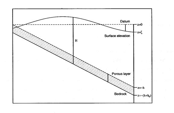
Figure 3-1. Schematic geometry of the porous medium beneath the sediment surface in ADAM model (Ip et al., 1998).

The combined open channel and porous medium system is described by

(3.8)

(3.9)

where is the transport in the open channel; is the porous medium transport; is the porosity, described by Darcy’s Law. The non-linear diffusion equation, Eq.(3.9), is discretized with linear finite elements by the Galerkin method in space (Appendix B) as

(3.10)

where q is the numerical implicity. The solution to the above equation is obtained iteratively in each time step.

3.4.1. Equations in the Wet (saturated) region where H > h₀ :

The total transport in the wet region is:

and

with the diffusion coefficient

and the velocity

where and

3.4.2. Equations in the Dry (unsaturated) region where H < h₀ :

The transport in the dry region is:

and

with the diffusion coefficient

and the velocity is

where and

3.5. The Program Structure

Main Program and Fixed Subroutines: ADAM2_v3.f is the core program, which performs all finite element assembly and solution operations with the backing of the fixed subroutines. ADAM2_v3.f reads formatted input files and writes a formatted echo file, the latter containing a summary of the input files and run data.

User Subroutine: A user-built subroutine must be linked to ADAM2_v3.f to specify the boundary forcing and the format in which the results are to be output.

Include File: The include file ADAM.DIM assigns values to parameters required for dimensioning purposes.

Input Files: The horizontal coordinates of each node in the mesh are given in a node file with the name ‘meshname’.nod. The bathymetry values of each node in the mesh are given in a bathymetry file named ‘meshname’.bat. The order of elements as they appear in the mesh is given in an element file named ‘meshname’.ele. The boundary node numbers where the tidal elevation forcing is applied are given in an elevation file named ‘meshname’.elv. The initial surface elevation and initial bottom friction coefficient at each node are given in two separate files named ‘meshname’//zinit.s2r and ‘meshname’//’simulation-name’.s2r, respectively.

All the files are in ASCII format. The input file formats are used without any change in the MATLAB routines, which were generated for post-processing purposes.

Figure 3-2. Structure of ADAM model.

3.5.1. Standard Output Files

‘meshname’.echo : This file contains useful information regarding the size of dimensional arrays, and the names of the input files.

‘meshname’.log : If the run is terminated due to dimensioning or boundary condition problems, log file gives a message describing the error.

v.v2r_e: This file is a 2-D, real valued, vertically-averaged horizontal velocity field. There are two header lines:

line 1: the geometric meshname

line 2: reserved for the user’s description of the file

Following these lines, there are NE lines of the form

I UOC(I) VOC(I)

Where: (UOC,VOC) are the (x, y) components of horizontal velocity in the open channel (MKS).

The loop is over the elements: I=1,NE

NE is the number of elements in the 2-D mesh.

q.v2r_e: A 2-D real valued vertically-averaged transport field. There are two header lines:

line 1: the geometric meshname

line 2: reserved for the user’s description of the file

Following these lines, there are NE lines of the form

I QUE(I) QVE(I)

Where: (QUE, QVE) are the (x, y) components of horizontal transport (MKS).

The loop is over the elements: I=1,NE

NE is the number of elements in the 2-D mesh.

z.s2r: A 2-D real valued scalar field (tidal elevations). There are two header lines:

line 1: the geometric meshname

line 2: reserved for the user’s description of the file

Following these lines, there are NN lines of the form

I ZN(I)

Where: ZN(I) is the scalar value at node I (MKS).

The loop is over the nodes: I=1,NN

NN is the number nodes in the 2-D mesh.

Any other output format is dependent on the user’s treatment of the User Subroutines. Residual velocity, residual transport and residual bottom stress at the end of each tidal cycle can be output in ASCII format.

The output files that are used in the MATLAB routines are created for visualization purposes. It is possible to create animation files with the output data in order to visualize the wetting/drying process in detail.