chapter 6

Modeling The m₂ tidal FLOW

for the entire great bay estuary

The principal lunar tide M₂, with a period of 12.42 hours, has important influences on the regional currents. Therefore, initial focus is centered on the M₂ harmonic constituent and its biharmonics (such as M₄ and M₆). The numerical ADAM model is tested for its ability to compute M₂ tidal dynamics in the Great Bay Estuary. The database of M₂ tidal elevations and currents from Swift and Brown (1983), is used in verification of the model and to test the assumptions made in the simulations.

 In this chapter, the bottom friction coefficient is fine-tuned for the M₂ tidal constituent until the model produced data that matched closely to the tidal analysis predicted for amplitude and phase data from Swift and Brown (1983).

6.1.            Computational Setup

The gbes4 mesh with 39617 linear triangular elements and 22140 nodes is used for the simulations. Bathymetry values are given at the corner nodes of each element. Boundary tidal forcing is applied at fifty-eight (58) nodes at the mouth of Portsmouth Harbor. M₂ tidal forcing with a period of 12.42 hrs is used at the Portsmouth Harbor open boundary. Four hundred (400) time steps are used per tidal cycle. The simulations are started with fluid at rest and are terminated after six M₂ tidal cycles at dynamic equilibrium. The simulation parameters are given in Table 6-1.

Table 6-1. Parameters used in ADAM model simulation of the Great Bay Estuary.

 

6.2.            Tidal Boundary Forcing at Portsmouth Harbor

M₂ tidal forcing is specified as the Dirichlet elevation boundary condition across the open ocean boundary extending from Gerrish Island in the north, to Odiorne Point in the southeast (see Figure 5-1). The elevation boundary condition used to force the model at the open ocean boundary is predicted using the harmonic constant derived from two offshore stations near Cape Porpoise Harbor (43.383^o N, 70.432^o W) and Hampton Harbor, NH (42.54^o N, 70.49^o W). Interpolated amplitude and phase for M₂ tidal forcing time series is 1.30m and 321.1^o K, respectively.

The predicted time series starts five M₂ tidal cycles before September 1, 1975. The length of the M₂ forcing time series is six (6) M₂ tidal cycles (74.52 hrs.). It starts on August 29, 1975 9:54 (663201.9 in Julian hours) and ends on September 1, 1975 12:25:12 (663276.42 in Julian hours). 

6.3.            Bottom Friction Coefficient Adjustment for the Great Bay Estuary

In this chapter, a space-variable, depth-dependent bottom friction coefficient distribution is adjusted for the M₂ tidal forcing until the model results fitted closely to the predicted surface elevation amplitude and phase and cross-section averaged velocity data from Swift and Brown (1983). In all the test simulations, the simulation parameters given in Table 6-1 are used. The bottom friction coefficient distributions for different simulations are shown in Figure 6-1.

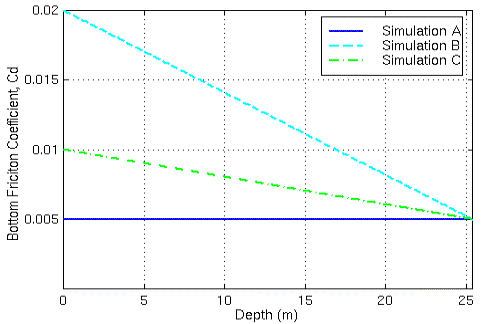
Figure 6-1. Space-variable, depth-dependent bottom friction coefficient distribution for simulations A, B and C.

 

6.4.            Statistical Analysis Methods

In order to compare the model results with the predicted time series  some statistical analysis has to be done. Definitions of some statistical analysis tools  that are used for comparative purposes are given below:

Correlation Coefficient: 

Correlation coefficient is a measure of the strength of the relationship between the model output and the predicted data. While variables having a high correlation coefficient do not guarantee a cause and effect relationship between the pair, having a high correlation is a necessary condition for such a relationship. Correlation coefficient is calculated as follows:

                      where C is the covariance matrix.

 

Normalized RMS (Root Mean Square) of Error: 

The Root Mean Square error is a measure of the deviation of the model output value from the predicted value. In Root Mean Square, the deviations are summed and then divided by the number of time periods in the time series. Finally, the square root of this quantity is evaluated. The Root Mean Square is used to quantitatively measure how closely the model output variable tracks the predicted data. The magnitude of the Root Mean Square error can be evaluated only by comparing it to the mean of the time series.

 

       where std is the standard deviation.

 

Skill:  Skill is defined as:

 

6.5.            Results for M₂ Forcing

Nine tidal stations, Seavey, T-11, T-12, T-13, T14A, T-14, T-16, T-UNH, and T-19 are used to make the surface elevation comparisons between model results and the predicted data from Swift and Brown (1983). Four stations, C-104, C-119, C124 and C-131 are used to make the cross-section averaged velocity comparisons between the model results and the predicted data from Swift and Brown (1983). The results from the simulations A, B, and C are compared with the predicted data from Swift and Brown (1983). Each simulation result is given below.

 

6.5.1.      Simulation A

This simulation is the starting point to find out the proper bottom friction coefficient distribution. First, a constant value bottom friction coefficient is used throughout the Great Bay Estuary to find the order of magnitude for the bottom friction coefficient.

 

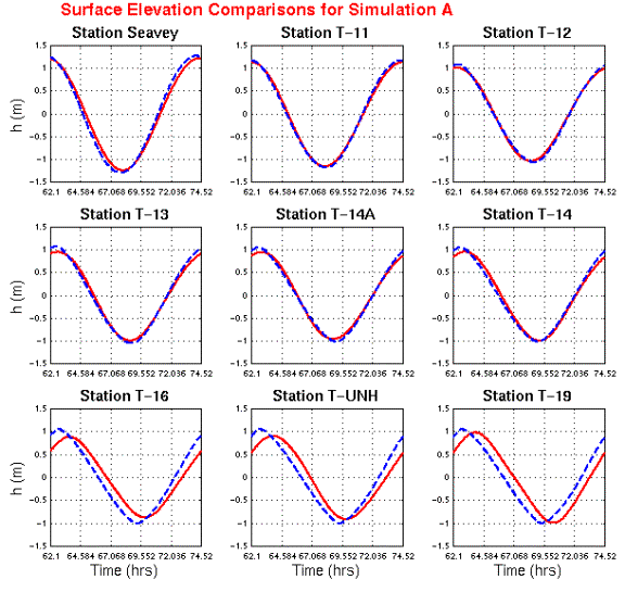
Figure 6-2. Simulation A: Surface elevation comparisons between the model–produced data and the tidal analysis predicted data. The tidal analysis predicted data are shown in solid red lines and model-produced data is shown in dashed blue lines.

 

The constant bottom friction works well in representing the flow between stations Seavey and T-14. In that region, the amplitudes and phases of the model predicted data matches with the tidal analysis predicted data. After station T-14, the elevations are not adequately damped to match the tidal analysis predictions and the model predicted data precedes the tidal analysis predicted data starting from station T-16.

The comparison of the model-produced, cross-section averaged velocities with the predicted data in Figure 6-3  shows that the model overpredicts the velocities with the specified bottom friction distribution.

 

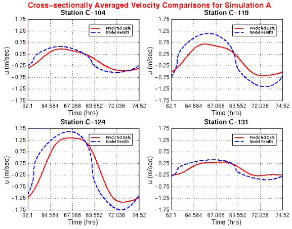
Figure 6-3. Simulation A: Comparison of cross-section averaged velocity values with tidal analysis predicted data. Solid red lines indicate tidal analysis predicted data and dashed blue lines indicate model-produced data.

 

 

6.5.2.      Simulation B

The results from the previous simulation indicate that the bottom friction coefficient values should be increased in order to decrease the velocities, which in turn will help to correct the phase differences. In this simulation, the bottom friction coefficient is increased and changed linearly with depth. The range for the friction coefficient is 0.005 and 0.02, the latter corresponding to the minimum depth.

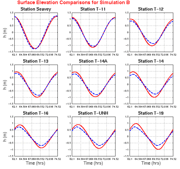
Figure 6-4. Simulation B: Surface elevation comparisons between the model–produced data and the tidal analysis predicted data. The tidal analysis predicted data are shown with solid lines and model-produced data is shown with dashed blue lines.

 

The bottom friction found is too high. Thus, the model predicted surface elevation amplitudes (beginning from station T-12) start damping too early.  However, the cross-section averaged velocity comparison in Figure 6-5 shows that the model-produced values at C-104 and C-131 compare well with the predicted data, but the model produced values at C-119 and C-124 do not match with the predicted data.

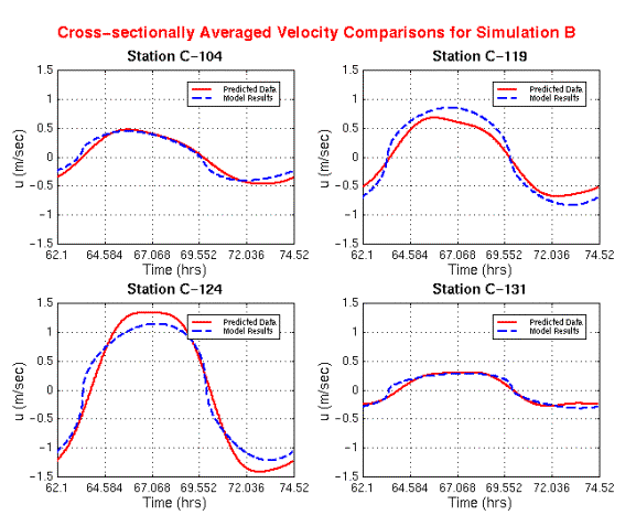
Figure 6-5. Simulation B: Comparison of cross-section averaged velocity values with tidal analysis predicted data. Solid lines indicate tidal analysis predicted data and dashed lines indicate model-produced data.

 

6.5.3.      Simulation C

In this simulation, the bottom friction coefficient is decreased in the deep channels in order to prevent early damping in the surface elevation amplitudes. The range for the friction coefficient is 0.005 and 0.01, the latter corresponding to the minimum depth. The maximum value for the bottom friction is reduced by half compared with simulation B.

 

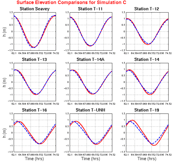
Figure 6-6. Simulation C: Surface elevation comparisons between the model–produced data and the tidal analysis predicted data. The tidal analysis predicted data are shown with solid red lines and model-produced data is shown with dashed blue lines.

 

The model predictions match with the tidal analysis predictions better than the previous two simulation results. However, there is still a phase difference between the model results and the tidal analysis predicted data. The model-produced data precedes the tidal analysis predictions starting from station T-16. The amplitudes on the other hand, are not damped too much and match closely with the tidal analysis predictions. 

The comparison for the cross-section averaged velocity values is shown in Figure 6-7. The model produced data matches the predicted data closely at stations C-104, C-124 and C-131. However, C-119 is a problem station.

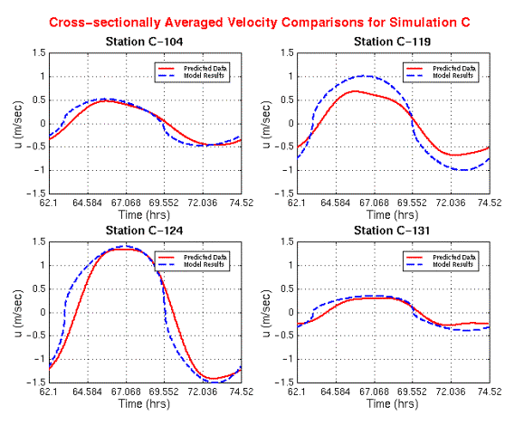
Figure 6-7.  Simulation C: Comparison of cross-section averaged velocity values with tidal analysis predicted data. Solid red lines indicate tidal analysis predicted data and dashed blue lines indicate model-produced data.

 

Comparison of different simulation results shows that when the phase of the model produced surface elevation time series agrees with the phase of the tidal analysis predicted surface elevation time series, the amplitudes of the model produced surface elevations time series do not agree with the amplitudes of the tidal analysis predicted surface elevation time series.

Statistical analysis results, including the correlation coefficient and the normalized Root Mean Square (RMS) values for each station, for simulations A, B and C are given in the following tables (Table 6-2 – Table 6-5).

 

Table 6-2. Correlation coefficient values at the current-meter stations.

 

 

Table 6-3. Correlation coefficient values at the surface elevation stations.

 

 

Table 6-4. Normalized Root Mean Square (RMS) values at the current-meter stations.

 

Table 6-5. Normalized Root Mean Square (RMS) values at the surface elevation stations.

 

6.6.            The gbes16 Mesh

The Great Bay section of the estuary, where the eelgrass distribution is most extensive, is the area of interest for exploring the frictional effects of eelgrass on the tidal flow. However, in the above simulations, the model produced flow was either damped too much or preceded the tidal analysis predicted data before reaching the Great Bay. At this stage, a strategic step was taken; the research was focused only on the tidal flow in the Great Bay section.

In order to resolve the flow in the Great Bay, the mesh is cut at Little Bay and a new boundary forcing is applied at the open boundary of the new mesh (see Figure 6-8). The boundary forcing is obtained by interpolating tidal analysis predicted amplitude and phase values at various stations in the estuary. The number of nodes is reduced from 22140 to 5657 and the number of elements is reduced from 39617 to 10526. Number of time steps per tidal cycles is reduced from 400 to 300. All these reductions help to reduce the computing time by 83%. In the new mesh, called the gbes16 mesh, the maximum element area is 8389.1m² and the minimum element area is 39.85m².

 

6.7.             Boundary Forcing for the gbes16 Mesh

The elevation time series used to force the model at the open boundary for the gbes16 mesh simulations is predicted using the harmonic constituents from Swift and Brown (1983).  First, the amplitude and phase values at all the stations (see Table 6-6) are interpolated to obtain the amplitude and phase values at the open boundary in Little Bay for each constituent. The amplitude and phase values found for the M₂ constituent are 0.85m and 27^oK, respectively. For the S₂ constituent the amplitude is 0.09m and the phase is 63^oK. For the N₂ constituent the amplitude is 0.18m and the phase is 347^oK.

Figure 6-8. The map of the surface elevation and cross-section averaged velocity stations and the open boundary in Little Bay.

 

The interpolated amplitude and phase values at the open boundary are used as input data together with the location west longitude (70.85) for the program TIDHAR. TIDHAR is a program that predicts the tidal forcing time series at a given location. The predicted boundary forcing time series for M₂, M₂S₂ and M₂S₂N₂ are shown in Figure 6-9.

 

Table 6-6. Amplitude and phase values for the significant sea level harmonic constituents at sea level stations (Swift and Brown, 1983). K is the local epoch.

	M2		S2		N2
Station	Amplitude  (m)	Phase     K (deg)	Amplitude (m)	Phase     K (deg)	Amplitude (m)	Phase     K (deg)
T-5	1.29	325	0.19	359	0.30	297
Seavey	1.20	333	0.17	8	0.28	306
T-11	1.12	336	0.15	10	0.25	308
T-12	1.00	346	0.15	29	0.23	318
T-13	0.95	352	0.14	32	0.22	322
T-14A	0.93	358	0.12	43	0.21	326
T-14	0.94	3	0.12	38	0.21	335
T-16	0.83	24	0.07	51	0.18	344
T-UNH	0.87	29	0.13	80	0.19	342
T-19	0.92	34	0.10	83	0.18	371

 

The predicted time series starts five M₂ tidal cycles before September 1, 1975. The length of M₂ forcing time series is six (6) M₂ tidal cycles (74.52 hrs.). It starts on August 29, 1975 at 9:54 am (663201.9 in Julian hours) and ends on September 1, 1975 at 12:25:12 pm (663276.42 in Julian hours).

The length of M₂S₂ is 36 M₂ tidal cycles (447.12 hours). It starts on August 29, 1975 at 9:54:00 am (663201.9 in Julian hours) and ends on September 17, 1975 at 1:02:24 pm  (663649.04 in Julian hours).

The length of M₂S₂N₂ time series is 108 M₂ tidal cycles (1341.36 hours). It starts on August 29, 1975 at 9:54 am (663201.9 in Julian hours) and ends on October 24, 1975 at 7:19:29 am  (664543.325 in Julian hours).

 

Figure 6-9. Time series of the boundary forcing for the gbes16 mesh. M₂ forcing is six M₂ tidal cycles (74.52 hrs) long whereas M₂S₂ forcing is 36 M₂ tidal cycles (447.12 hrs) and M₂S₂N₂ forcing is 108 M₂ tidal cycles (1341.36 hrs) long.

 

The Great Bay system is forced with the above-mentioned boundary forcing time series for the M₂, M₂S₂ and M₂S₂N₂ tidal forcing in the following chapters.