2008 Election Model

2008 Election Model

A Monte Carlo Electoral Vote Simulation

Updated: Nov. 3, 2008

FINAL PROJECTION:

Obama wins by 76-64m votes; 367-171 EV (median); 365.3 expected; 53-45% vote share

The Election Model (EM) assumes as a base case that a fraud-free election is held today – and that current polls reflect the true vote. The model projects that Obama will win the Electoral vote by 367-171 and the True Vote by 76-64m. The final projected vote share is Obama 53.1- McCain 44.9%- Other 2.0%. The state poll aggregate vote share matched the national average tracking poll to within 0.2%.

The model projects that Obama will carry 30 states + DC:

CA CO CT DE FL HI IL IA ME MD / MA MI MN MO MT NV NH NJ NM NY / NC ND OH OR PA RI VT VA WA WI

In May, the 2008 Election Calculator (EC) projected that Obama would win the True Vote by 71-59m (54.1-44.7%).

For the 2008 EC to match the EM, its estimate of returning 60.5m returning Kerry and 51.6m Bush voters had to be accurate.

The EC used 12:22am 2004 NEP vote shares to calculate the projections.

In other words, the 2008 EC and EM confirmed that Kerry won a landslide (see below).

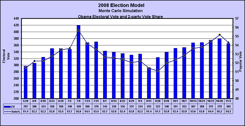
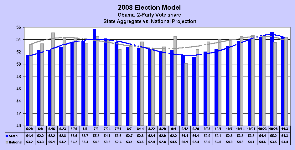
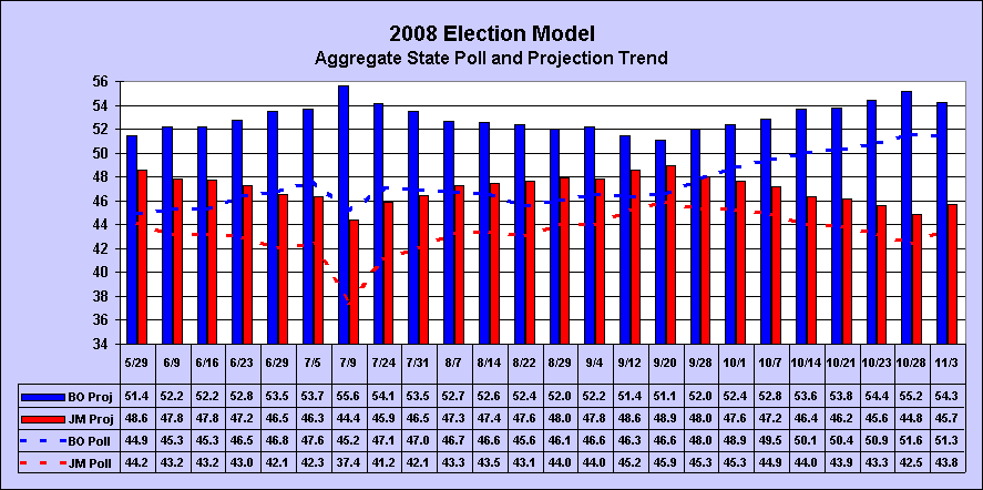
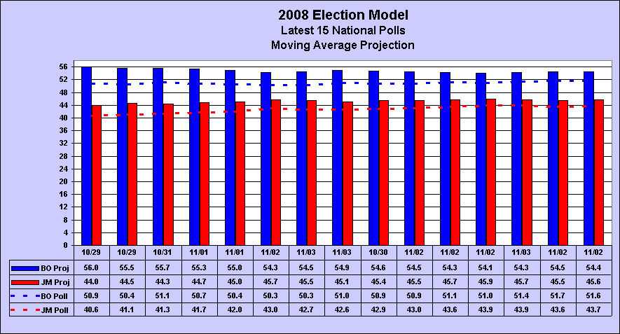
These graphs display the trend from May 29-Nov. 3: Electoral vote and projected vote share trend and State vs. National vote share projection trend.

The average of recent state polls is entered in the database. The EM assumes that 60% of the undecided voters will break to Obama (base case). The undecided vote allocation (UVA) is based on the assumption that Obama is the challenger and McCain is running for Bush’s third term (GWB is not the most popular of incumbents). The EM base case allocates a conservative 60% of the undecided vote to Obama; most pollsters typically use 70-90%, depending on the incumbent’s approval rating. Bush is at 22% and McCain 45%.

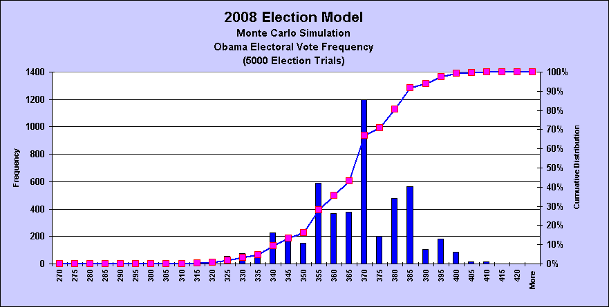
The model projects five vote share scenarios of undecided voter allocations (UVA) ranging from 40-90%. Obama won the base case scenario with an average 365.8 EV. The median and mode were 367. Even in the worst-case 40% UVA scenario Obama won all 5000 election trials.

The Monte Carlo mean EV (365.8) matched the theoretical expected EV (365.3), illustrating the Law of Large Numbers (LLN): 5000 simulated election trials were required for the MEAN EV to CONVERGE to the THEORETICAL EV (the simulation is in the “long run”). It is computational overkill to perform a meta analysis requiring the calculation of millions of EV combination scenarios in order to calculate the win probabilities.

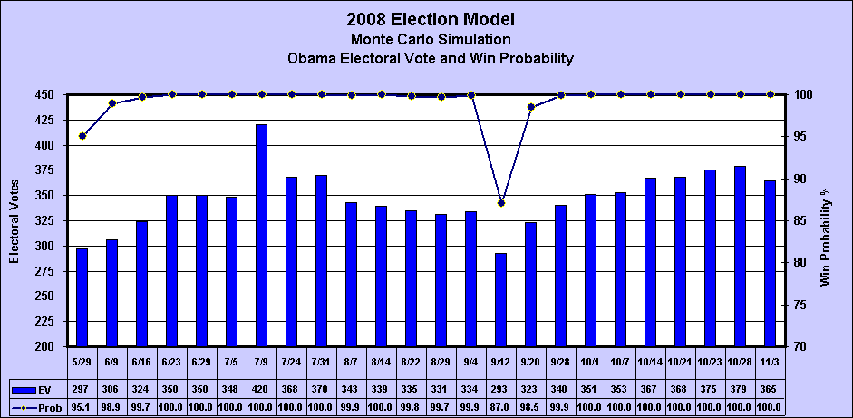
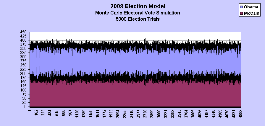
Obama exceeded 360 EV in 3333 of 5000 Monte Carlo election trial simulations, so he has a 66.7% probability of winning at least 360 EV. The Monte Carlo simulation is displayed in this Electoral Vote Simulation Frequency chart. Note that ALL 5000 election trials are to the right of the 270 mark; therefore Obama’s win probability is 100%.

2008 Election Model

Final Monte Carlo Simulation

TruthIsAll

Updated:

11/3/08

10:13 AM

Assumptions:

143.0

Votes cast

138.7

Recorded

(in millions)

3.0%

Uncounted

4.3

75%

to Obama

2.0%

3rd party

2.9

Nader, Barr, McKinney et al

60%

Undecided Voters (UVA) allocated to Obama

National Model

Obama

McCain

Other

Margin

Tracking Poll Avg (%)

51.1

43.9

5.0

7.3

Projected True Vote %

52.9

45.1

2.0

7.9

Projected True Vote (mil)

75.7

64.4

2.9

11.3

Proj. Recorded Vote %

52.3

45.7

2.1

6.6

(True Vote less Uncounted)

Proj. Recorded Vote (mil)

72.5

63.4

2.9

9.1

Proj. 2-party True Vote %

54.1

45.9

0.0

8.3

State Model

Aggregate Poll Avg (%)

51.3

43.8

4.9

7.6

Projected True Vote %

53.1

44.9

2.0

8.2

Projected True Vote (mil)

75.9

64.2

2.9

11.7

Proj. Recorded Vote %

52.4

45.5

2.1

6.9

(True Vote less Uncounted)

Proj. Recorded Vote (mil)

72.7

63.2

2.9

9.5

Proj. 2-party True Vote %

54.3

45.7

0.0

8.6

Electoral Vote Snapshot

Poll Leader

367

171

Before UVA

Projected Leader

370

168

After UVA

Expected EV

365.29

172.71

EV = ∑ (Win probability (i) * EV(i)), i=1,51 states

Monte Carlo Electoral Vote Simulation (5000 election trials)

Mean

365.81

172.19

Average

Median

367

171

Middle value

Mode

367

171

Most likely

Maximum

414

124

Minimum

294

244

Obama Electoral Vote Win Probabilities

Electoral Vote

320

330

340

350

360

370

380

390

400

410

420

Trial Wins > EV

4969

4832

4668

4218

3333

2270

1072

380

Change in Trial Wins

137

164

450

885

1063

1198

692

330

Prob. Trial Wins > EV

99.38%

96.64%

93.4%

84.4%

66.7%

45.4%

21.4%

7.6%

1.00%

0.06%

0.00%

STATE POLL MODEL

NATIONAL POLL MODEL

ELECTORAL VOTE

Wtd Avg

2-Party

Actual

Moving

2-Party

Actual

Expected

Polls

Current

Proj

Average

Current

Proj

Value

11/3/08

60% UVA

Obama

51.3

54.0

54.28

53.08

51.1

53.8

54.14

52.94

365.3

McCain

43.8

46.0

45.7

44.9

43.9

46.2

45.9

45.1

172.7

map

11/01/04

75% UVA

Kerry

47.9

50.5

51.8

51.1

47.8

50.6

51.8

51.3

337

Bush

46.9

49.5

48.2

47.9

46.6

49.4

48.2

47.8

201

map

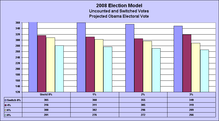
Impact of Uncounted and Switched Votes on Obama 2-party Aggregate Vote Share and Expected EV

Uncounted

Switched

Vote

4.0%

52.0

311

51.8

305

51.6

319

8.0%

49.8

276

49.6

272

49.4

266

10.0%

48.7

251

48.5

247

48.3

242

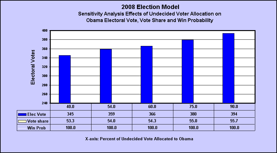
Impact of Undecided Voter Allocation (UVA) on Obama 2-party Aggegate Vote Share and Expected EV

Current

Base case

UVA

40%

54.0%

60%

75%

90%

Projected 2-Party Vote Share

Obama

53.3

54.0

54.3

55.0

55.7

McCain

46.7

46.0

45.7

45.0

44.3

MoE

Obama Popular Vote Win Probability (Normdist)

1.0%

100.0

2.0%

99.9

100.0

3.0%

98.4

99.5

99.7

99.9

100.0

Obama Electoral Vote: Monte Carlo Simulation (5000 election trials)

Mean

345.0

359.0

365.8

379.5

393.8

Median

347

362

367

381

396

Mode

367

381

396

Maximum

395

406

414

421

445

Minimum

289

294

317

333

Electoral Vote Win Probability

Trial Wins

5000

Probability

100.0

95% EV Confidence Interval

Upper

381

394

399

409

421

Lower

309

324

333

350

367

States Won

Obama

POLLING ANALYSIS AND PROJECTIONS

National Model

http://www.realclearpolitics.com/epolls/2008/president/us/general_election_mccain_vs_obama-225.html

0.47

State aggregate vs. National vote share correlation

Current Poll Average

7-Poll Moving Average

Projected Moving Average Vote (60% UVA)

Poll

Date

Sample

MoE

Obama

McCain

Other

Spread

Obama

McCain

Spread

WinPr

Obama

McCain

Spread

WinPr

Research2k

11/02

1100LV

2.95%

51.1

43.9

7.3

100.0

54.1

45.9

8.3

100.0

Gallup

11/02

2847RV

1.84%

51.1

43.7

7.4

100.0

54.2

45.8

8.5

100.0

Zogby

11/02

1201LV

2.83%

51.0

44.0

7.0

100.0

54.0

46.0

8.0

100.0

Hotline/FD

11/02

882LV

3.30%

50.7

43.7

7.0

99.8

54.1

45.9

8.1

100.0

Rasmussen

11/02

3000LV

1.79%

51.3

43.1

8.1

99.2

54.6

45.4

9.3

99.7

ABC/WP

11/02

2446RV

1.98%

51.1

42.7

8.4

100.0

54.8

45.2

9.7

100.0

Battleground

10/30

1000LV

3.10%

50.1

43.0

7.1

96.6

54.3

45.7

8.5

99.1

NBC/WSJ

11/02

1011LV

3.08%

50.3

43.0

7.3

100.0

54.3

45.7

8.6

100.0

CNN

11/01

1017LV

3.07%

50.4

42.0

8.4

99.9

55.0

45.0

9.9

100.0

Pew

11/01

2587RV

1.93%

50.7

41.7

9.0

100.0

55.3

44.7

10.5

100.0

CBS

10/31

1005LV

3.09%

51.1

41.3

9.9

99.9

55.7

44.3

11.4

100.0

Marist

10/29

543LV

4.21%

50.4

41.1

9.3

92.6

55.5

44.5

11.0

99.0

FOX News

10/29

924LV

3.22%

50.9

40.6

10.3

98.6

56.0

44.0

12.0

99.6

Ipsos

10/27

831LV

3.40%

51.3

40.3

11.0

100.0

56.3

43.7

12.7

100.0

Pew

10/26

1325RV

2.69%

51.6

39.9

11.7

100.0

56.7

43.3

13.4

100.0

50.45

43.91

5.64

6.55

51.75

40.25

8.00

11.50

Total

50.80

42.93

6.27

7.87

2-party

54.20

45.80

0.00

8.39

State Model

http://www.electoral-vote.com/

http://www.realclearpolitics.com/epolls/maps/obama_vs_mccain/#data

Poll MoE

3.0%

LATEST STATE POLLS

2004 PROJECTIONS, EXIT POLLS, ACTUALS

Kerry

Recorded Vote

Obama vs

Obama

KEY STATES

Proj.

Unadj.

Recd

Deviation from

Kerry

Flip (*)

Obama

McCain

Spread

2pty Proj.

WinProb

(within MoE)

Vote

Proj.

Exit

2pty Proj.

States

Last Poll

Popular

51.34

43.77

7.57

54.28

100.0

Allocation

51.02

51.98

48.27

2.75

3.71

2.76

Date

Electoral

367

171

196

370

365.3

Percent

Rank

337

252

128

10/28

(25)

37.8

0.0

41.3

41.8

36.8

4.4

5.0

(4.0)

10/30

(18)

41.2

0.0

39.0

40.2

35.5

3.5

4.7

1.7

10/30

(4)

48.4

14.8

6.0

48.0

44.5

44.4

3.6

0.1

(0.1)

10/31

(7)

47.0

2.5

1.4

49.8

45.2

44.5

5.2

0.6

(3.3)

10/31

62.4

100.0

55.0

60.1

54.3

0.7

5.8

6.9

10/30

53.4

98.7

3.2

50.0

50.1

47.0

3.0

3.1

2.9

CO*

10/22

61.4

100.0

55.8

62.3

54.3

1.4

8.0

5.2

9/13

90.6

100.0

85.5

90.6

89.2

(3.7)

1.4

4.6

10/28

65.4

100.0

57.0

61.3

53.3

3.7

8.0

7.9

11/2

51.4

82.0

22.7

51.5

51.0

47.1

4.4

3.9

(0.6)

FL*

10/30

(3)

49.0

25.7

10.8

45.8

42.0

41.4

4.4

0.6

2.8

9/20

71.0

100.0

51.8

58.1

54.0

(2.3)

4.1

18.8

9/17

(29)

36.0

0.0

37.5

32.3

30.3

7.2

2.0

(2.0)

11/1

61.8

100.0

56.3

56.6

54.8

1.4

1.8

5.1

11/2

(2)

49.6

39.7

9.2

40.5

40.4

39.3

1.2

1.1

8.6

11/1

58.2

100.0

53.8

50.7

49.2

4.5

1.5

4.0

IA*

10/28

(17)

42.0

0.0

38.5

37.2

36.6

1.9

0.5

3.0

11/1

(14)

43.4

0.0

42.0

39.9

39.7

2.3

0.2

0.9

10/29

(10)

46.0

0.4

48.3

43.5

42.2

6.0

1.3

(2.8)

11/1

56.6

100.0

57.5

55.6

53.6

3.9

2.0

(1.4)

9/20

60.0

100.0

55.5

59.6

55.9

(0.4)

3.7

4.0

10/28

59.8

100.0

70.0

65.8

61.9

8.1

3.9

(10.7)

11/1

58.4

100.0

53.5

54.4

51.2

2.3

3.2

4.4

11/2

55.4

100.0

54.3

55.7

51.1

3.2

4.6

0.7

10/29

(11)

45.0

0.1

46.5

49.4

39.8

6.3

9.3

(2.0)

11/2

51.2

78.3

10.6

49.3

49.0

46.1

3.1

2.9

1.5

MO*

11/2

51.0

74.3

2.9

40.5

37.3

38.6

1.9

(1.3)

10.0

MT*

9/30

(19)

41.2

0.0

36.5

37.0

32.7

3.8

4.4

4.2

11/2

54.0

99.6

1.2

49.8

52.8

47.9

1.9

5.0

3.8

NV*

10/30

56.0

100.0

50.8

57.2

50.2

0.5

7.0

4.8

10/30

59.2

100.0

55.3

57.5

52.9

2.3

4.6

3.5

10/31

54.2

99.7

0.6

49.8

53.0

49.0

0.7

4.0

NM*

10/28

67.0

100.0

59.3

64.5

58.4

0.9

6.1

7.3

11/2

50.8

69.9

14.4

48.5

49.5

43.6

4.9

6.0

1.8

NC*

10/29

(1)

50.2

55.2

2.9

41.8

34.6

35.5

6.3

(0.9)

8.0

ND*

11/2

53.4

98.7

7.2

51.5

54.0

48.7

2.8

5.3

1.4

OH*

10/29

(29)

35.8

0.0

35.5

33.8

34.4

1.1

(0.6)

(0.2)

10/30

59.0

100.0

53.8

53.0

51.3

2.4

1.7

4.8

11/2

55.0

99.9

53.0

55.1

50.9

2.1

4.2

1.5

10/1

59.8

100.0

61.3

62.1

59.4

1.8

2.7

(2.0)

10/29

(10)

45.4

0.1

43.5

45.8

40.9

2.6

4.9

1.4

10/31

(9)

45.8

0.3

45.8

35.9

38.4

7.3

(2.6)

(0.5)

10/22

(14)

43.6

0.0

48.5

43.2

42.5

6.0

0.6

(5.4)

10/21

(10)

45.2

0.1

39.3

42.0

38.2

1.0

3.8

5.5

10/30

(24)

39.2

0.0

28.5

28.1

26.0

2.5

2.2

10.2

10/26

62.4

100.0

57.5

66.5

58.9

(1.4)

7.6

4.4

11/2

52.8

96.6

6.2

47.8

49.8

45.5

2.3

4.4

4.6

VA*

10/31

58.2

100.0

54.3

56.8

52.8

1.4

4.0

3.5

10/26

(8)

46.8

1.8

0.6

48.8

40.2

43.2

5.6

(3.0)

(2.5)

10/29

57.6

100.0

54.0

52.1

49.7

4.3

2.4

3.1

WI*

10/29

(23)

39.2

0.0

32.8

32.6

29.1

3.7

3.5

6.0

These graphs display the polling and projection trends (Refresh the screen for the latest update):

Aggregate state poll and projection trend

National 5-poll moving average projection

State vs. National vote share projection trend

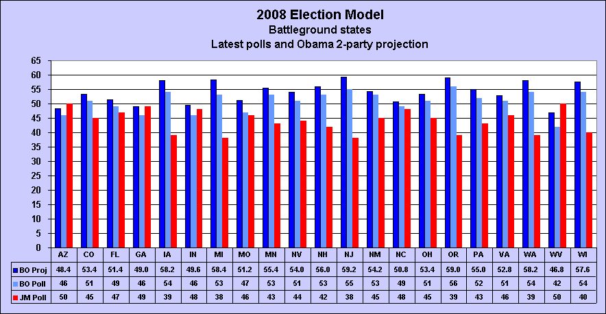
Battleground state polls and projections

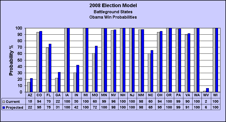
Battleground state win probability

Electoral vote and win probability trend

Electoral vote and projected vote share trend

Undecided voter allocation and win probability

Monte Carlo Electoral Vote Simulation Trials

Electoral Vote Simulation Frequency

Effect of uncounted and switched votes on the projected vote share

Effect of uncounted and switched votes on the expected electoral vote

Polling data source:

Electoral-vote.com

RealClearPolitics.com

The 2008 Election Calculator Model confirms the 2004 and 2008 Election Model (and vice-versa).

In May, the 2008 Election Calculator projected that Obama would win the True Vote by 71-59m (54.1-44.7%).

Estimated vote share

2004 Turnout Votes Mix Obama McCain Other

DNV - 17.2 13.1% 59% 40% 1%

Kerry 95% 60.5 46.2% 89% 10% 1%

Bush 95% 51.6 39.4% 11% 88% 1%

Other 95% 1.6 1.2% 70% 11% 19%

Total 113.7 130.9 100% 54.1% 44.7% 1.2%

130.9 70.8 58.5 1.6

Checking the 2004 Election Calculator (EC) True Vote and the 2008 Election Model (EM) projections

On Nov.3, 2008 the following test was performed:

The 12:22am 2004 NEP vote shares were input to the 2008 EC.

In the 2008 EM, 75% UVA and 3^rd party 1% share were input to match 2004 EC assumptions.

The resulting 2008 EC projection closely matched the EM (to within 0.2%).

Therefore, the EC 2004 vote shares and weighting mix are also confirmed and therefore must be fairly accurate.

The 2008 EC could only be accurate (and match the EM) if the input estimate of returning 2004 Bush and Kerry voters was also accurate.

The model estimates 60m returning Kerry voters and 51.6m returning Bush voters.

Given a 75% UVA and 1% to Other, the EC projects Obama will win by 78.3-63.8 million votes, assuming a fraud-free election.

Note that the base case EM is 60% UVA and 2% Other

2004 Election Calculator

Voted Est. 2004 Calculated True Vote (12:22am NEP)

In 2000 Turnout Votes Mix Kerry Bush Other

DNV - 25.6 20.4% 57% 41% 2%

Gore 95% 49.7 39.5% 91% 8% 1%

Bush 95% 46.6 37.1% 10% 90% 0%

Other 95% 3.8 3.0% 64% 17% 19%

Total 100.1 125.7 100.0% 53.2% 45.4% 1.4%

True Vote 125.7 66.9 57.1 1.7

Deviation from Recd Vote 3.4 +4.9% -5.3% +0.4%

Unadjusted Exit Poll 52.0% 47.0% 1.0%

Votes Cast 125.7 65.4 59.1 1.3

Deviation from True Vote -1.2% +1.6% -0.4%

Recorded Vote share 48.3% 50.7% 1.0%

Recorded Vote 122.3 59.0 62.0 1.2

Deviation from Exit Poll -3.7% +3.7% 0.0%

2008 Election Calculator

12:22am NEP vote share

2004 Turnout Votes Mix Obama McCain Other

DNV - 29.9 20.8% 57% 41% 2%

Kerry 95% 60.6 42.2% 91% 8% 1%

Bush 95% 51.6 35.9% 10% 90% 0%

Other 95% 1.6 1.1% 64% 17% 19%

Total 113.7 143.7 100% 54.5% 44.4% 1.1%

143.7 78.3 63.8 1.5

2008 Election Model (75% UVA) 54.3% 44.7% 1.0%

78.0 64.3 1.4

2008 Election Model (60% UVA) 53.1% 44.9% 2.0%

75.9 64.2 2.9

Projected Vote Shares, Electoral Votes and Win Probabilities

There are many electoral vote forecasting models. The following Monte Carlo models gave a 100% Obama win probability.

DeSart and Holbrook

The Oct. 16 model run projected that Obama would win 52.85% of the national 2-party vote, 354-184 EV with a 99.99% win probability.

University of Illinois

http://election08.cs.uiuc.edu/

The simulation model was developed by computer science and political science students.

270towin

An interactive model of 1000 Monte Carlo election trials.

http://www.270towin.com/simulation/

Franklin & Marshall College

Calculates a 99.98% probability that Sen. Barack Obama will win. But executing 50 million election trials is extreme overkill. Only 5000 are necessary.

http://politicalwire.com/archives/2008/10/31/simulation_shows_obama_will_win.html

Electoral-vote.com and RealClearPolitics assign the full electoral vote to the state poll leader regardless of the spread; they avoid using state win probabilities in calculating the EV and do not allocate undecided voters. Therefore, if the polls are tied or McCain slightly ahead in swing states, their EV totals understate the EM electotoral vote projection for Obama.

The discrepancy in win probabilities between the Election Model (EM) and fivethirtyeight.com (538) is due to differences in methodology.

. 538 attempts to forecasts the Election Day result; the EM assumes the election is held today.

. 538 weights state poll projections based on pollster rankings and many other factors; the EM does not rank pollsters.

Ranking pollsters based on prior performance is not just overkill; it introduces a built-in, counter-intuitive bias. For example, the final Rasmussen 2004 poll was quite accurate in projecting the recorded vote. But since the election was rigged and the recorded vote was not equal to the true vote, should he get a high rating? If Rasmussen included a fraud component in his polling model, he would have been correct, but he did not. On the other hand, Zogby projected that Kerry would win - and he won the True Vote. Because the election was stolen, Zogby gets a bad rap. Go figure. In 2000 (before rigged machines were institutionalized by HAVA) Zogby correctly predicted the recorded vote and Rasmussen was way off.

The 538 site is very well done with lots of polling information. But it is my firm belief that their model suffers from complexity overkill and feature creep. The First Law of Analytical Model Building is KISS: Keep It Simple Stupid. My opinion is based on 30 years experience as a quantitative analyst and model builder/programmer in scientific, engineering and financial applications. I also have several advanced math degrees.

The 1988-2004 Election Calculator

The Final National Exit Poll was forced to match the recorded vote using impossible weightings.

In the Final, 43% of 2004 voters (52.6m) were former Bush 2000 voters; 37% were Gore voters.

But Bush only had 50.5m votes in 2000.

Approximately 2.5m died and another 2.5m did not return to vote.

Therefore, only 45.5m Bush 2000 voters could have returned to vote in 2004.

The Final overstated the Bush vote by 7 million in order to match a corrupt miscounted vote.

The 2004 True Vote calculation was based on an estimated 100.1m returning 2000 voters, calculated as:

Total votes cast in 2000 (110.8m) less voter mortality (5.4m) times 95% turnout (100.1m).

Vote shares were based on the 12:22am National Exit Poll.

The model determined that Kerry won by 66.9-57.1 million.

Kerry did slightly better (53.2%) than the unadjusted state exit poll (52.0%) aggregate.

The results indicate that 5.4m votes (8.0% of Kerry’s total) were switched from Kerry to Bush.

Election Model Calculations

The projected vote share is equal to the latest poll plus the undecided voter allocation.

V (i) = Poll (i) + UVA (i).

The probability P (i) of winning state (i) is based on the projected state vote share V (i).

It is calculated using the Excel Normal distribution function, assuming a 3.0% MoE for a typical 2-state average (1200 total sample size):

P (i) = NORMDIST (V (i), 0.5, .03/1.96, true).

The expected state electoral vote is the product of the win probability and electoral vote.

The total expected EV is given by the summation formula:

EV = ∑ P (i) * EV (i), where i= 1, 51 states.

The Electoral Vote Win probability is based on a 5000 election-trial Monte Carlo Simulation.

The EV win probability is the number of winning election trials/5000.

Why Election Model projections differ from the Media, Academia and the Bloggers

There are a variety of election forecasting models used in academia, the media and internet election sites. The corporate MSM (CNN, MSNBC, FOX, CBS, etc.) sponsors national polls to track the “horserace” and state polls to calculate the electoral vote.

The EM uses Monte Carlo (MC) simulation method to calculate the probability of winning the electoral vote. Monte Carlo is widely used to analyze diverse risk-based models when an analytical solution is impractical or impossible. The EM is updated weekly based on the latest state and national polls. The model projects the popular and electoral vote, assuming both clean and fraudulent election scenarios. The EM allocates the electoral vote based on the state win probability in calculating a more realistic total Expected EV.

Corporate MSM pollsters and media pundits use state and national polling data. Electoral vote projections are misleading since they are calculated based on the latest state polls regardless of the spread; the state poll leader gets all of its electoral votes. This is statistically incorrect; they do not consider state win probabilities. And there is no adjustment for the allocation of undecided voters.

For example, assume that McCain leads by 51-49% in each of five states with a total of 100 electoral votes. Most models would assign the 100 EV to McCain. But Obama could easily win one or more of the states since his win probability is 31%. The 2008 Election Model would allocate 31 EV to Obama and 69 to McCain.

Bloggers also track state and national polls and do not adjust for undecided voters. A few use Monte Carlo simulation but the EV win probabilities and frequency distributions are NOT consistent with the polling data. Either the state win probabilities and/or the simulation algorithm is incorrect.

Academic regression models predict the popular vote but are run months prior to the election. They are typically based on economic and political factors rather than state or national polling data. They do not project the electoral vote. In 2004, virtually all of them forecast Bush to win by 5-10%. But since the election was stolen, the models had to be wrong – they didn’t factor election fraud as an independent variable in the regression. In fact, they never even mentioned the F-word in describing their methodologies.

Fixing the polls: Party ID, Voted in 2000, RV vs. LV

Most national and state polls are sponsored by the corporate MSM. Gallup, Rasmussen and other national polls recently increased the Republican Party ID percentage weighting. This had the immediate effect of boosting McCain’s poll numbers. But there are 11 million more registered Democrats than Republicans. USA Today/Gallup changed the poll method from RV to LV right after the Republican convention. Party-ID weights were manipulated to favor McCain as well.

There is a consistent discrepancy between Registered Voter (RV) and Likely Voter (LV) Polls. The Democrats always do better in RV polls. No wonder: Since 1988, Democratic presidential candidates have won new voters by an average 14% margin.

The manipulation of polling weights is nothing new. Recall that the 2004 and 2006 Final National Exit Polls weightings were adjusted to match the recorded vote miscount. But all category cross-tabs had to be changed, not just Party ID. Of course, the Final Exit Poll (state and national) is always matched to the recorded vote even though it may be fraudulent – as it was in 2000, 2002, 2004 and 2006.

In 2004, the 12:22am National Exit Poll (NEP) had a 38/35 Democrat/Republican Party ID mix. Kerry won the NEP by 51-48%. The weighting mix was changed to 37/37 in the Final NEP in order to force a match to the recorded vote miscount. Likewise, the Gore/Bush “Voted 2000” weights were changed from 39/41 to 37/43 in the Final NEP. Bush was the official winner by 50.7- 48.3% with 286 EV.

The final 2004 Election Model projection indicated that Kerry would win 337-201 EV with 51.8% of the 2-party vote. In their Jan. 2005 report, exit pollsters Edison-Mitofsky provided the average exit poll discrepancy for each state based on 1250 total precincts. Kerry won the unadjusted aggregate state exit poll vote share by 52.0-47.0% (2-party 52.5%) with 337 electoral votes - exactly matching the Election Model!

In the 2006 midterms, the 7pm NEP had a 39/35 Democratic/Republican weighting mix. The Democrats won the NEP by 55-43%. But the weights were changed to 38/36 in the Final NEP in order to match the 52-46% recorded vote; the Dem 12% margin was cut in half. Once again, the “Voted 2004” weights were transformed: from Bush/Kerry 47/45 at 7pm to 49/43 in the Final. The landslide was denied; 10-20 Dem seats were stolen.

The “dead heat” claimed by pollsters, bloggers and the media is a canard- unless they are factoring fraud into their models and not telling us. The media desperately wants a horserace and fail to adjust polls for undecided and newly registered voters. They avoid McCain’s gaffes, flip-flops and plagiarisms while he supports the most unpopular president in history.

The Great Election Fraud Lockdown: Uncounted, Stuffed and Switched Votes

Professional statistical organizations, media pundits and election forecasters who projected a Bush victory never discuss Election Fraud. On the contrary, a complicit media has been in a permanent election fraud lockdown as it relentlessly promotes the fictional propaganda that Bush won BOTH elections. They want you to believe that Democrats always do better in the exit polls because Republican voters are reluctant responders. But they never consider other, more plausible explanations – such as uncounted and stuffed ballots. Millions of mostly Democratic ballots are uncounted, spoiled and stuffed in every election and favored a Bush I and II in 1988, 1992, 2000 and 2004. That’s why the Democratic True vote (and exit poll share) is always greater than the Recorded vote. Read more here

- In most states, total votes cast exceeded votes recorded (uncounted ballots exceeded stuffed). In Florida, Ohio and 10 other states, total votes recorded exceeded votes cast (ballot stuffing exceeded uncounted ballots).

- The majority (70-80%) of uncounted ballots are in Democratic minority precincts. According to the 2000 Vote Census, 5.4m of 110.8m votes cast (4.9%) were uncounted (approximately 4.0m were Gore votes).

- In 2004, Bush won the recorded vote by 62-59m. But 3.4m of 125.7m votes cast were uncounted (2.7%) and 2.5m were for Kerry. If they were counted, the recorded Bush 3.0m margin is cut in half, 62.9 - 61.5m. And that’s before vote rigging.

- Media-commissioned exit polls indicated that Kerry won by 52-47%.

- The exit pollsters never explained why mathematically impossible weights were used in the Final National Exit Poll to force a match the recorded vote count.

- Historically, challengers have won 60-90% of the undecided vote (UVA) when the incumbent was unpopular. In 2004, final state and national polls had the race nearly tied at 47% and Bush had a 48% approval rating. That’s one reason why the Gallup poll projected that Kerry would win 88% of the late undecided vote.

The 2004 Election Model allocated 75% of the undecided vote to Kerry as the base case scenario. It projected that Kerry would have an expected 337 electoral votes with 51.8% of the two-party vote and a 99% electoral vote win probability.

In the Three-Card Monte con, the mark is tricked into betting that he can find the money card among three face-down cards. A rigged election is the vote scam equivalent of Three-Card Monte. What you see in the exit polls is not what you get in the recorded count; the recorded vote is never equal to the True vote. In this con game, the voter is the mark. Any model which correctly calculates the True vote is doomed to fail in a rigged election.

Calculating the Expected Electoral Vote and Win Probability

Most election forecasting blogs and academics and the media employ the latest state polls as input to their models but don’t use basic probability, statistics and simulation concepts in forecasting the electoral vote and corresponding win probability. A meta-analysis or simulation is not required to calculate the expected electoral vote. Of course, the individual state vote projections depend on the particular forecasting method used. With all due respect to Professor Sam Wang, his Meta-Analysis program is an unnecessarily complex combinatorial algorithm when compared to Excel and Monte Carlo simulation for calculating the expected Electoral Vote and Win Probability.

The Excel-based Election Model is straightforward. After updating the database for the latest state polling data, the vote shares are projected by allocating undecided voters. The normal distribution function calculates the corresponding state win probability. The expected state EV is the product of the win probability and electoral vote. The sum of the 51 state expected EVs is the total expected EV. The final step is to calculate the EV Win Probability. The EM uses a 5000-trial Monte Carlo simulation. MC is widely used for analyzing complex systems when an analytical solution is prohibitive due to the virtually infinite number of possible combinations of risk-based variables (i.e. state win probabilities).

The winner of the election trial is the candidate who has at least 270 EV. The electoral vote win probability is simply the number of winning election trials divided by 5000.

The convergence of the simulated mean to the theoretical formula mean EV illustrates the Law of Large Numbers (LLN) and shows that 5000 election trials are sufficient in order to derive an accurate win probability.

Other links:

Confirmation of A Kerry Landslide
Election Fraud Analytics and Response to the TruthIsAll FAQ

2004 Registered Voter (RV) vs. Likely Voter (LV) Polls

Excel models available for download:

The Election Calculator: 1988-2004
2004 Interactive Simulation Model
A Polling Simulation Model
2000-2004 County Vote Database